AGRP
Asteraceae Genomic Research Platform
Asteraceae Genomic Research Platform
# Download via command line
wget ftp://ftp.ncbi.nlm.nih.gov/blast/executables/blast+/LATEST/ncbi-blast-2.13.0+-x64-linux.tar.gz

# Unzip
tar -zxvf ncbi-blast-2.13.0+-x64-linux.tar.gz

# Rename
mv ncbi-blast-2.13.0+-x64-linux blast

# Environment variable settings
# Edit the ~/.bashrc file and add the following line at the end:
export PATH=/home/local/Software/blast/bin:$PATH

# Configuration effective
source ~/.bashrc
# 1. Makeblastdb (Format Database):
makeblastdb -in db.fasta -dbtype prot -parse_seqids -out dbname

# Parameter description:
# -in: the sequence file to be formatted
# -dbtype: database type, prot or nucl
# -out: database name
# -parse_seqids: parse sequence identifier (recommended to add)

# 2. Blastp (Protein vs Protein):
blastp -query seq.fasta -out seq.blast -db dbname -outfmt 6 -evalue 1e-5 -num_descriptions 10 -num_threads 8

# 3. Blastn (Nucleic vs Nucleic):
blastn -query seq.fasta -out seq.blast -db dbname -outfmt 6 -evalue 1e-5 -num_descriptions 10 -num_threads 8

# 4. Blastx (Nucleic vs Protein):
blastx -query seq.fasta -out seq.blast -db dbname -outfmt 6 -evalue 1e-5 -num_descriptions 10 -num_threads 8

# Output Format (m8) Columns:
# 1. Query id        2. Subject id      3. Identity %
# 4. Alignment len   5. Mismatches      6. Gap openings
# 7. Q.start         8. Q.end           9. S.start
# 10. S.end          11. E-value        12. Bit score
# When comparing the makeblastdb library with blast, pay attention to the parameters (dbtype), whether the protein file (prot) is used or the nucleic acid file (nucl).
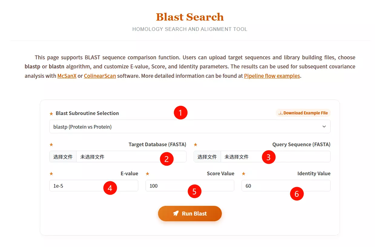
1.Select the desired Blast subroutine Choose between blastp (Protein vs Protein) or blastn (Nucleotide vs Nucleotide) from the dropdown menu.
2.Upload the Target Database file Click to upload the library file you want to search against (must be in FASTA format).
3.Upload the Query Sequence file Click to upload the specific sequence file you want to analyze (must be in FASTA format).
4.Enter the E-value threshold Input the expectation value cutoff (default is 1e-5) to filter significant hits.
5.Input the Score Value Enter the minimum alignment score required (default is 100).
6.Input the Identity Value Enter the minimum percentage of identity required for a match (default is 60).
7.Click the "Run Blast" button Submit the form to start the homology search and alignment process.
#Unzip
tar zxf diamond-linux64.tar.gz
#Rename
mv diamond ~/bin
#Environment variable settings
echo 'PATH=$PATH:/root/bin' >> ~/.bashrc
#Configuration effective
source ~/.bashrc
## linux command:
# Build a database
diamond makedb --in nr --db nr
## Sequence alignment
# Nucleic acid
diamond blastx --db nr -q reads.fna -o dna_matches_fmt6.txt
# Protein
diamond blastp --db nr -q reads.faa -o protein_matches_fmt6.txt
# When comparing the diamond makedb library with diamond blast, pay attention to the parameters, whether the protein file is used or the nucleic acid file.
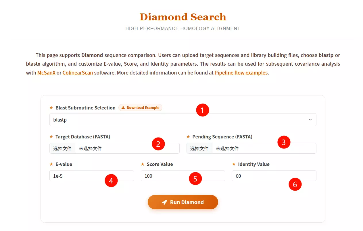
1.Select the desired Blast subroutine Choose between blastp (Protein vs Protein) or blastx (Translated Nucleotide vs Protein) from the dropdown menu.
2.Upload the Target Database file Click to upload the reference library file you want to search against (must be in FASTA format).
3.Upload the Pending Sequence file Click to upload the query sequence file you want to analyze (must be in FASTA format).
4.Enter the E-value threshold Input the expectation value cutoff (default is 1e-5) to filter significant hits.
5.Input the Score Value Enter the minimum alignment score required (default is 100) to filter results.
6.Input the Identity Value Enter the minimum percentage of identity required for a match (default is 60).
7.Click the "Run Diamond" button Submit the form to start the high-performance homology alignment process.
# Unzip:
unzip MCScanX-master.zip

# Compile
make
## Preparation:
# 1. Put the gff file and blast file into the same folder.
# 2. The gff file should be the merged result of two species' gff files.
# 3. The blast file and gff file must share the same prefix name (e.g., se_so.gff and se_so.blast).

# Run MCScanX
MCScanX se_so

# Plotting covariance points (Dot Plot)
java dot_plotter -g se_so.gff -s se_so.collinearity -c dot.ctl -o dot.PNG
# Error 1: "msa.cc:289:9: error: ‘chdir’ was not declared in this scope"
# Solve 1: Open "msa.cc", add #include <unistd.h> at the top.

# Error 2: "dissect_multiple_alignment.cc:252:44: error: ‘getopt’ was not declared in this scope"
# Solve 2: Open "dissect_multiple_alignment.cc", add #include <getopt.h> at the top.

# Error 3: "detect_collinear_tandem_arrays.cc:286:17: error: ‘getopt’ was not declared in this scope"
# Solve 3: Open "detect_collinear_tandem_arrays.cc", add #include <getopt.h> at the top.
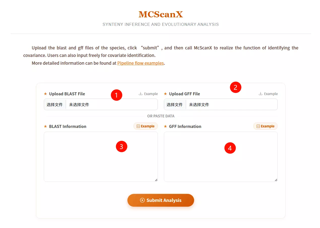
1.Upload the BLAST File Click to upload the pairwise alignment file (usually generated by BLASTP) which contains the homologous gene pairs.
2.Upload the GFF File Click to upload the General Feature Format file that defines the physical positions of the genes on the chromosomes.
3.Input BLAST Information (Optional) Alternatively, if you do not have a file, paste the raw BLAST result data directly into this text area.
4.Input GFF Information (Optional) Alternatively, if you do not have a file, paste the raw GFF coordinate data directly into this text area.
5.Click the "Submit Analysis" button Submit the form to run the MCScanX algorithm for synteny inference and evolutionary analysis.
# 1. Extracting gene pairs from BLAST results
cat ath_chr2_indica_chr5.blast | get_pairs.pl --score 100 > ath_chr2_indica_chr5.pairs

# 2. Masking of highly repetitive loci
cat ath_chr2_indica_chr5.pairs | repeat_mask.pl -n 5 > ath_chr2_indica_chr5.purged

# 3. Estimate maximum gap length
max_gap.pl --lenfile ath_chrs.lens --lenfile indica_chrs.lens --suffix purged

# 4. Detect covariate fragments
block_scan.pl --mg 321000 --mg 507000 --lenfile ath_chrs.lens --lenfile indica_chrs.lens --suffix purged
#!/bin/sh
do_error()
{
    echo "Error occured when running $1"
    exit 1
}

echo "Start to run the working example..."
echo

echo "* STEP1 Extract pairs from BLAST results"
echo "  We should parse BLAST results and extract pairs of anchors (genes in this example) satisfying our rule (score >= 100)."
cat ath_chr2_indica_chr5.blast | get_pairs.pl --score 100 > ath_chr2_indica_chr5.pairs || do_error get_pairs.pl
echo

echo "* STEP2 Mask highly repeated anchor"
echo "  Highly repeated anchors which are mostly generated by continuous single gene duplication events make those colinear segements vague to be detected. We mask them off using a very simple algorithm."
cat ath_chr2_indica_chr5.pairs | repeat_mask.pl -n 5 > ath_chr2_indica_chr5.purged || do_error repeat_mask.pl
echo

echo "* STEP3 Estimate maximum gap length"
echo "  Use pair files with repeats masked to estimate mg values which will be used to detected colinear blocks."
max_gap.pl --lenfile ath_chrs.lens --lenfile indica_chrs.lens --suffix purged || do_error max_gap.pl
echo

echo "* SETP4 Detect blocks from pair file(s)"
echo "  Everything's ready do scan at last."
block_scan.pl --mg 321000 --mg 507000 --lenfile ath_chrs.lens --lenfile indica_chrs.lens --suffix purged || do_error block_scan.pl
echo

echo "Now ath_chr2_indica_chr5.blocks contains predicted colinear blocks."
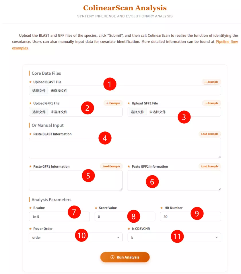
1.Upload the BLAST File Click to upload the pairwise sequence alignment file (generated by BLAST) containing the homologous gene pairs.
2.Upload the GFF1 File Click to upload the General Feature Format file describing the gene positions for the first genome (Reference/Query).
3.Upload the GFF2 File Click to upload the General Feature Format file describing the gene positions for the second genome (Target/Subject).
4.Paste BLAST Information (Optional) If you don't have a file, paste the raw BLAST alignment text data directly into this area.
5.Paste GFF1 Information (Optional) If you don't have a file, paste the raw GFF coordinate data for the first genome into this area.
6.Paste GFF2 Information (Optional) If you don't have a file, paste the raw GFF coordinate data for the second genome into this area.
7.Enter the E-value threshold Input the expectation value cutoff (default is 1e-5) to filter out insignificant alignment hits.
8.Input the Score Value Enter the minimum alignment score required (default is 0) to accept a match.
9.Input the Hit Number Enter the maximum number of top hits to consider for analysis (default is 30).
10.Select Position or Order Choose "pos" to use physical chromosomal positions (bp) or "order" to use gene rank order for collinearity calculations.
11.Select Is CDSVCHR Choose "is" or "no" to determine if the software should strictly match Coding Sequence (CDS) IDs to Chromosome IDs.
12.Click the "Run Analysis" button Submit the form to execute ColinearScan and identify conserved gene blocks.
# Official download address:
https://ngdc.cncb.ac.cn/tools/paraat
# "ParaAT.pl" is the running script. You can use it directly after downloading and unpacking.
# Either add the unpacked path to your environment variable or use the absolute path.

# Dependency Tools Required:
# 1. Protein comparison tools (install at least one): clustalw2, mafft, muscle, etc.
# 2. KaKs_Calculator (https://ngdc.cncb.ac.cn/tools/kaks)

# Run ParaAT Command:
ParaAT.pl -h test.homologs -n test.cds -a test.pep -p proc -m muscle -f axt -g -k -o result_dir

# Parameter Explanation:
# -h: Homologs file
# -n: CDS file
# -a: Protein (pep) file
# -p: Number of processors (threads)
# -m: Aligner to use (e.g., muscle)
# -f: Output format (e.g., axt)
# -k: Calculate Ka/Ks (calls KaKs_Calculator)
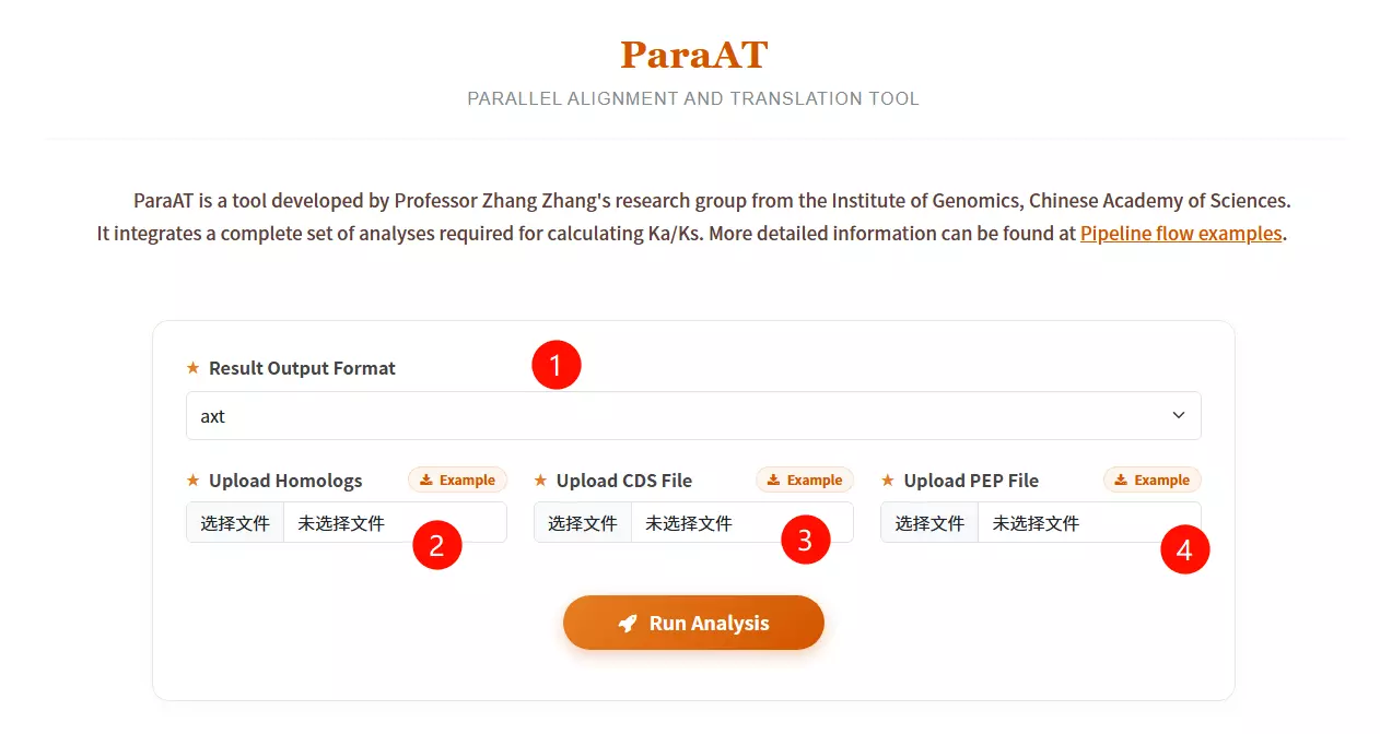
1.Select the Result Output Format Choose the desired file format for the alignment output (e.g., axt, fasta, paml, codon, or clustal) from the dropdown menu.
2.Upload the Homologs file Click to upload the text file containing the list of homologous gene pairs or groups to be analyzed.
3.Upload the CDS Sequence file Click to upload the Coding DNA Sequence (CDS) file corresponding to the gene list (must be in FASTA format).
4.Upload the Protein Sequence file Click to upload the Peptide/Protein (PEP) sequence file corresponding to the gene list (must be in FASTA format).
5.Click the "Run Analysis" button Submit the form to start the parallel alignment and translation process.
# Official download address:
https://ngdc.cncb.ac.cn/biocode/tools/BT000001
# Unzip
unzip KaKs_Calculator3.0.zip

# Compile KaKs
cd KaKs_Calculator3.0 && make
# Main programs generated: KaKs, KnKs, AXTConvertor

# Environment setup
# Add the path to your environment variables.
# Note: This tool often works in conjunction with ParaAT.
# See ParaAT installation here: [Go to ParaAT Section]
# 1. Prepare input files
# test.cds: DNA sequence of each gene
# test.pep: Protein sequences for each gene
# proc: A file containing a number indicating the number of CPU calls (e.g., just write '8' in it)

# 2. Start analysis (Calling KaKs_Calculator via ParaAT)
ParaAT.pl -h test.homolog -n test.cds -a test.pep -p proc -m mafft -f axt -g -k -o result_dir

# Parameter explanation:
# -h : homologous gene name file
# -n : file of specified nucleic acid sequences (CDS)
# -a : specified protein sequence file (PEP)
# -p : specifies the file containing thread count
# -m : specifies the comparison tool (clustalw2 | t_coffee | mafft | muscle)
# -g : remove codons with gaps
# -k : use KaKs_Calculator to calculate kaks values
# -o : output directory
# -f : format of the output comparison file (AXT is standard for KaKs_Calculator)
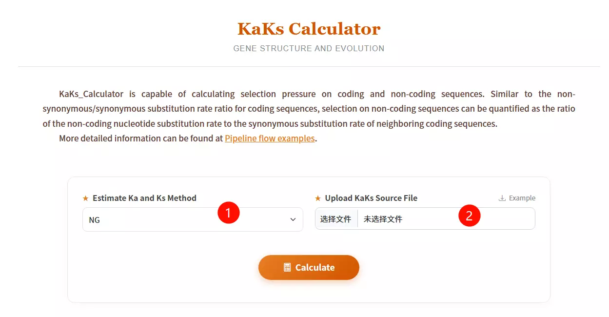
1.Select the Estimate Ka and Ks Method Choose the desired calculation algorithm (e.g., NG, YN, GY, MA) from the dropdown menu to determine how substitution rates are estimated.
2.Upload the KaKs Source File Click to upload the sequence alignment file you want to analyze (must be in AXT format as shown in the example).
3.Click the "Calculate" button Submit the form to initiate the calculation of non-synonymous (Ka) and synonymous (Ks) substitution rates.
# Online web server:
http://www.ebi.ac.uk/Tools/hmmer/

# Official local download:
http://hmmer.org/
# 1. Basic Usage:
# hmmbuild builds a profile HMM from a multiple sequence alignment (MSA).
hmmbuild [-options] <hmmfile_out> <msafile>

# 2. Input/Output Description:
# <msafile> : The input file must be a multiple sequence alignment.
#             Supports formats: CLUSTALW, SELEX, GCG MSF, etc.
# <hmmfile_out> : The output HMM database file (usually .hmm extension).

# 3. Common Options:
# hmmbuild usually automatically detects input type (DNA/Protein).
# You can force the sequence type:
# --amino : Force input to be interpreted as protein sequences.
# --dna   : Force input to be interpreted as DNA sequences.
# --rna   : Force input to be interpreted as RNA sequences.
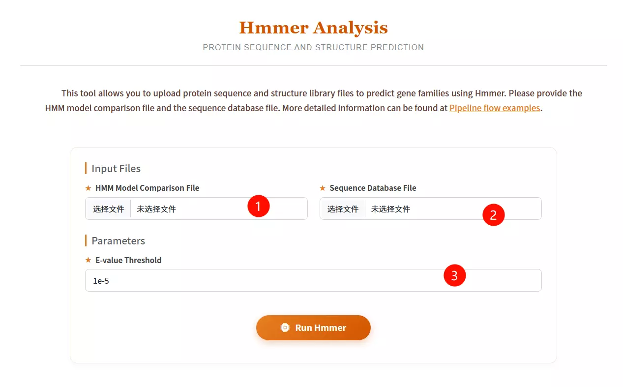
1.Upload the HMM Model Comparison File Click to upload the Hidden Markov Model file (usually with a .hmm extension) representing the protein family or domain profile you wish to use as a query.
2.Upload the Sequence Database File Click to upload the protein sequence library file you want to search against (must be in FASTA format).
3.Enter the E-value Threshold Input the expectation value cutoff (default is 1e-5) to filter out statistically insignificant matches and control the sensitivity of the search.
4.Click the "Run Hmmer" button Submit the form to initiate the profile-based homology search and structure prediction process.
# 1. Download Database Files (EBI FTP)
wget https://ftp.ebi.ac.uk/pub/databases/Pfam/current_release/Pfam-A.hmm.gz
wget https://ftp.ebi.ac.uk/pub/databases/Pfam/current_release/Pfam-A.hmm.dat.gz
wget https://ftp.ebi.ac.uk/pub/databases/Pfam/current_release/Pfam-A.seed.gz
wget https://ftp.ebi.ac.uk/pub/databases/Pfam/current_release/Pfam-A.full.gz

# 2. Unzip
gunzip Pfam-A.hmm.gz

# 3. Format the Pfam database (using hmmpress from HMMER package)
hmmpress Pfam-A.hmm
# Run the program (Example)
nohup pfam_scan.pl \
  -fasta /your_path/masp.protein.fasta \
  -dir /your_path/PfamScan/Pfam_data \
  -outfile masp_pfam \
  -cpu 16 &

# Result Analysis (Output Columns Description):
# (1) seq_id     : Transcript ID (IDs not in list are non-coding)
# (2) hmm start  : Starting position of the domain match
# (3) hmm end    : End position of the domain match
# (4) hmm acc    : ID of the Pfam domain (Accession)
# (5) hmm name   : Name of the Pfam domain
# (6) hmm length : Length of the Pfam domain model
# (7) bit score  : The score of the alignment
# (8) E-value    : Significance. (Filter condition usually: Evalue < 0.001)
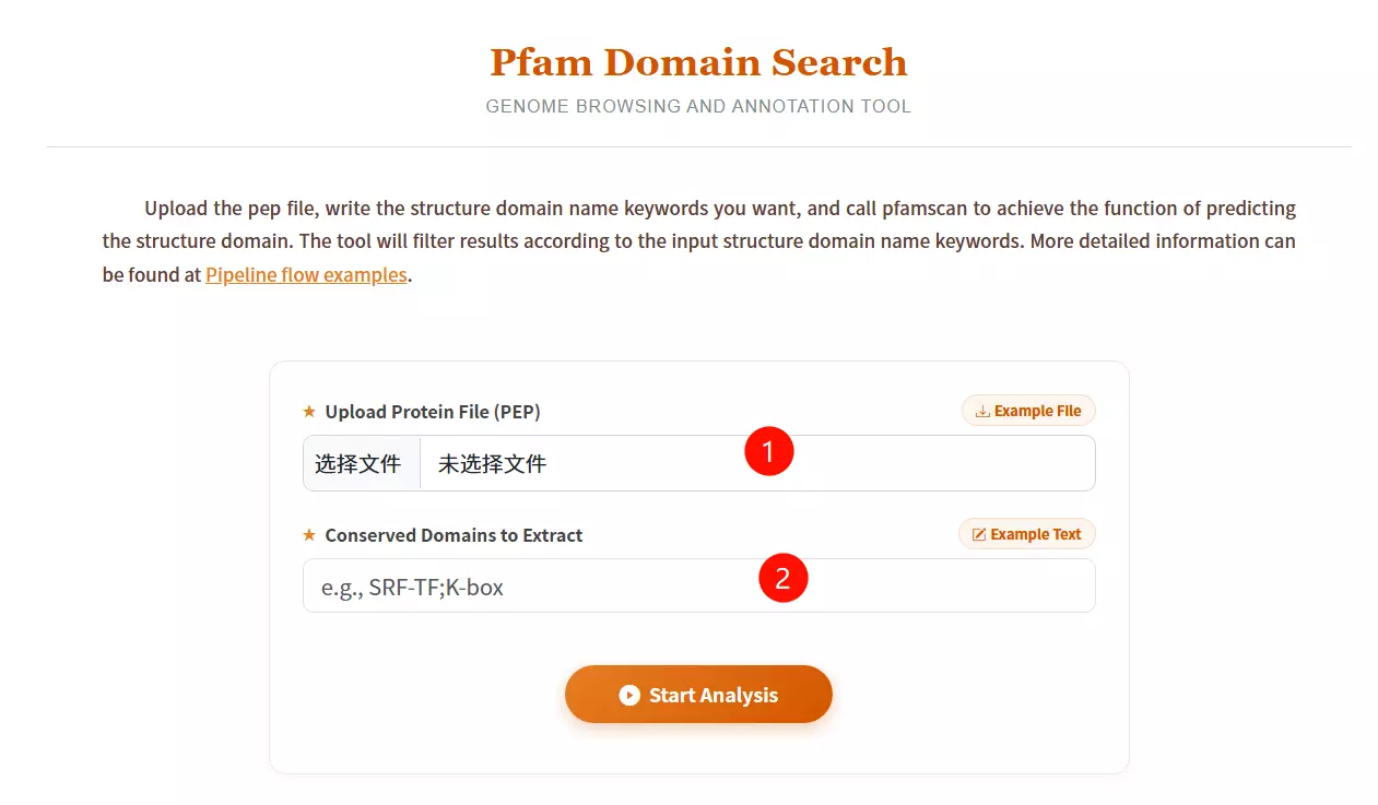
1.Upload the Protein File (PEP) Click to upload the protein sequence file you want to analyze for domain prediction (must be in FASTA format).
2.Enter Conserved Domain Keywords Input the specific structural domain names you wish to filter or extract (e.g., SRF-TF;K-box), separating multiple keywords with semicolons.
3.Click the "Start Analysis" button Submit the form to execute pfamscan and retrieve the domain prediction results.
# Prerequisites: Perl version 5.10.1+ is required.
# If you need to install Perl manually:
tar zxvf perl.tar.gz
cd /yourpath/perl
./Configure -des -Dprefix=/yourpath/perl_Dusethreads
make && make test && make install
# Add to PATH: export PATH=/yourpath/perl_Dusethreads/bin:$PATH

# Installing MEME:
tar zxf meme.tar.gz
cd meme_5.5.4
./configure --prefix=/yourpath/meme --with-url=http://meme-suite.org --enable-build-libxml2 --enable-build-libxslt
make
make test
make install

1.Upload the Target Database file Click to upload the sequence file containing the data in which you want to discover motifs (must be in FASTA format).
2.Select the Sequence Type Choose the biological type of your input sequences (Protein, DNA, or RNA) from the dropdown menu.
3.Select the Distribution Pattern Choose the expected occurrence of the motif per sequence: "Zero or One Occurrence" (ZOOPS), "One Occurrence" (OOPS), or "Any Number of Repetitions" (ANR).
4.Input the Number of Motifs Enter the maximum number of distinct motifs you want the software to identify (default is 3).
5.Input the Minimum Width Enter the minimum length (in residues or nucleotides) allowed for a single motif (default is 2).
6.Input the Maximum Width Enter the maximum length (in residues or nucleotides) allowed for a single motif (default is 10).
7.Click the "Find Motifs" button Submit the form to run the MEME algorithm and start the motif discovery process.
# The program is intended to search for CpG islands in sequences.

# 1. Min length of island to find:
# Searching CpG islands with a length (bp) not less than specified.

# 2. Min percent G and C:
# Searching CpG islands with a composition not less than specified.

# 3. Min CpG number:
# The minimal number of CpG dinucleotides in the island.

# 4. Min gc_ratio [P(CpG) / expected P(CpG)]:
# The minimal ratio of the observed to expected frequency of CpG dinucleotide in the island.

# 5. Extend island:
# Extending the CpG island if its length is shorter than required.
Search parameters:  len: 200   %GC: 50.0   CpG number: 0   P(CpG)/exp: 0.600   extend island: no   A: 21   B: -2
Locus name:  9003..16734 note="CpG_island (%GC=65.4, o/e=0.70, #CpGs=577)"
Locus reference:   expected P(CpG): 0.086   length: 25020
    20.1%(a)  29.9%(c)  28.6%(g)  21.4%(t)   0.0%(other)

                FOUND 4 ISLANDS
  #     start      end   chain   CpG    %CG    CG/GC    P(CpG)/exp     P(CpG)    len
  1      9192    10496     +     161   73.0    0.847   0.927( 1.44)    0.123    1305
  2     11147    11939     +      87   69.2    0.821   0.917( 1.28)    0.110     793
  3     15957    16374     +      57   79.4    0.781   0.871( 1.60)    0.137     418
  4     14689    15091     +      49   74.2    0.817   0.887( 1.42)    0.122     403
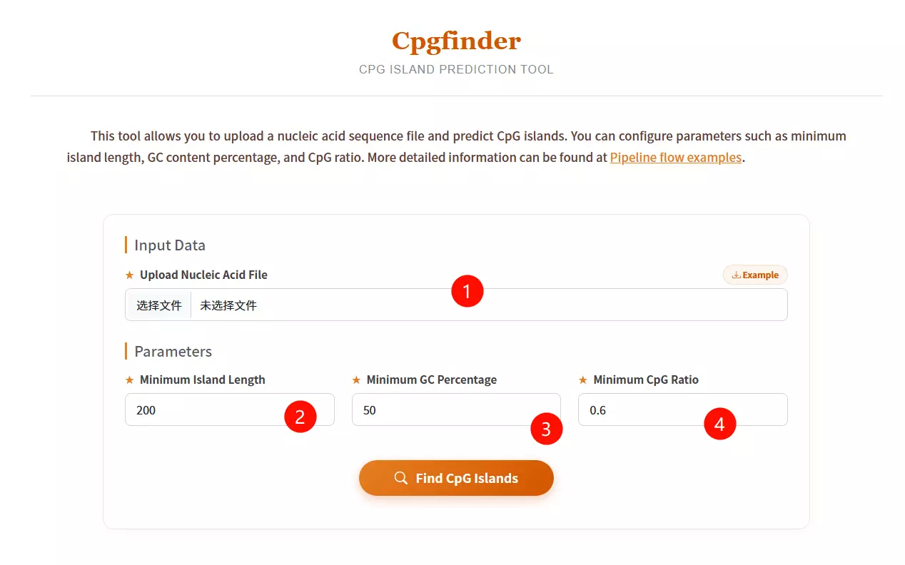
1.Upload the Nucleic Acid Sequence file Click to upload the DNA sequence file you want to analyze for CpG island prediction (e.g., in FASTA or plain text format).
2.Input the Minimum Island Length Enter the minimum length in base pairs required for a region to be defined as a CpG island (default is 200 bp).
3.Input the Minimum GC Percentage Enter the minimum percentage of Guanine and Cytosine content required within the sliding window (default is 50%).
4.Input the Minimum CpG Ratio Enter the minimum threshold for the observed-to-expected CpG dinucleotide ratio (default is 0.6).
5.Click the "Find CpG Islands" button Submit the form to execute the algorithm and identify genomic regions matching the specified criteria.
# Install directly with conda:
conda install codonw

# Run:
codonw

# Expected Initial Menu Output:
# Welcome to CodonW  for Help type h
# Initial Menu
# Option
# (1) Load sequence file
# (3) Change defaults
# (4) Codon usage indices
# (5) Correspondence analysis
# (7) Teach yourself codon usage
# (8) Change the output written to file
# (9) About C-codons
# (R) Run C-codons
# (Q) Quit
 Codon usage indices Options:
 ( 1) {Codon Adaptation Index       (CAI)          }
 ( 2) {Frequency of OPtimal codons  (Fop)          }
 ( 3) {Codon bias index             (CBI)          }
 ( 4) {Effective Number of Codons   (ENc)          }
 ( 5) {GC content of gene           (G+C)          }
 ( 6) {GC of silent 3rd codon posit.(GC3s)         }
 ( 7) {Silent base composition                     }
 ( 8) {Number of synonymous codons  (L_sym)        }
 ( 9) {Total number of amino acids  (L_aa )        }
 (10) {Hydrophobicity of protein    (Hydro)        }
 (11) {Aromaticity of protein       (Aromo)        }
 (12)  Select all
 (X)   Return to previous menu
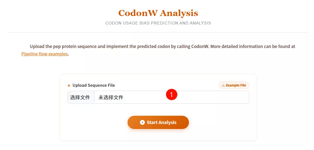
1.Upload the Sequence File Click to upload the specific sequence file you want to analyze (must be in FASTA format).
2.Click the "Start Analysis" button Submit the form to start the CodonW prediction and analysis process.
conda install iqtree
# 1. Automatic model selection and tree inference:
iqtree -s example.phy -m MF -mtree -T AUTO

# 2. Specify a substitution model (e.g., GTR+I+G):
iqtree -s example.phy -m GTR+I+G

# 3. ModelFinder + Tree + UltraFast Bootstrap (1000 replicates):
iqtree -s example.phy -m MFP -b 1000 -T AUTO

# 4. ModelFinder + Tree + UltraFast Bootstrap + BN-NNI search:
iqtree -s example.phy -m MFP -B 1000 --bnni -T AUTO
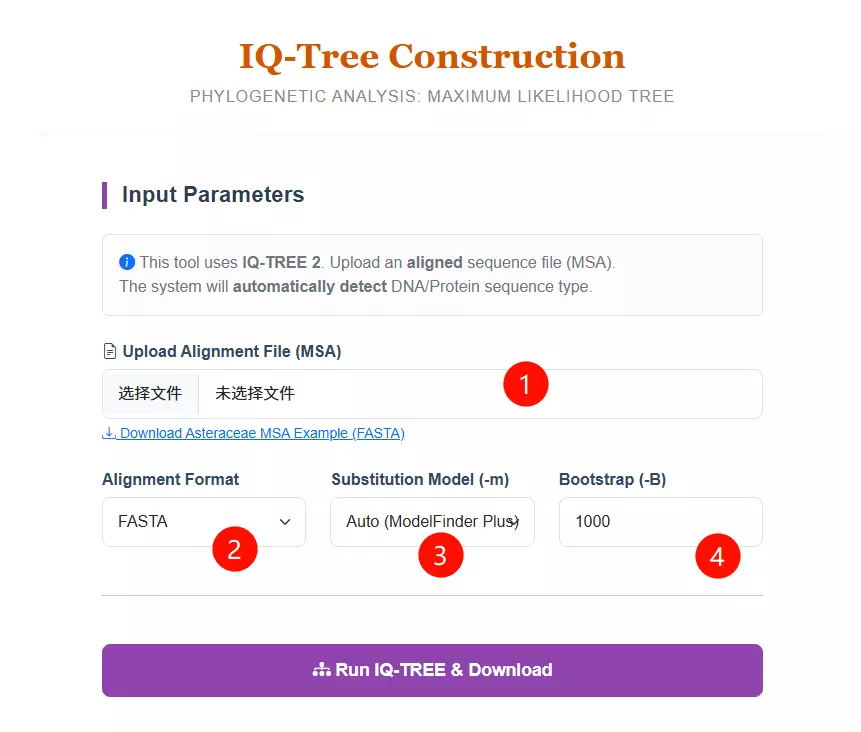
1.Upload the Alignment File Click to upload your Multiple Sequence Alignment (MSA) file. Note that this must be an aligned sequence file (DNA or Protein), not raw sequences.
2.Select the Alignment Format Choose the specific format of your uploaded file (FASTA, PHYLIP, or NEXUS) from the dropdown menu to ensure correct parsing.
3.Select the Substitution Model Choose a specific evolutionary substitution model (e.g., GTR+G for DNA, LG+G for Protein) or keep the default "Auto (ModelFinder Plus)" to let the system automatically detect the best-fit model.
4.Input the Bootstrap Value Enter the number of bootstrap replicates (default is 1000) to calculate the statistical support for the tree branches.
5.Click the "Run IQ-TREE & Download" button Submit the form to start the Maximum Likelihood tree construction process.
conda install fasttree
# Nucleotide alignment:
fasttree -nt nucleotide_alignment_file > tree_file

# Protein alignment:
fasttree protein_alignment_file > tree_file
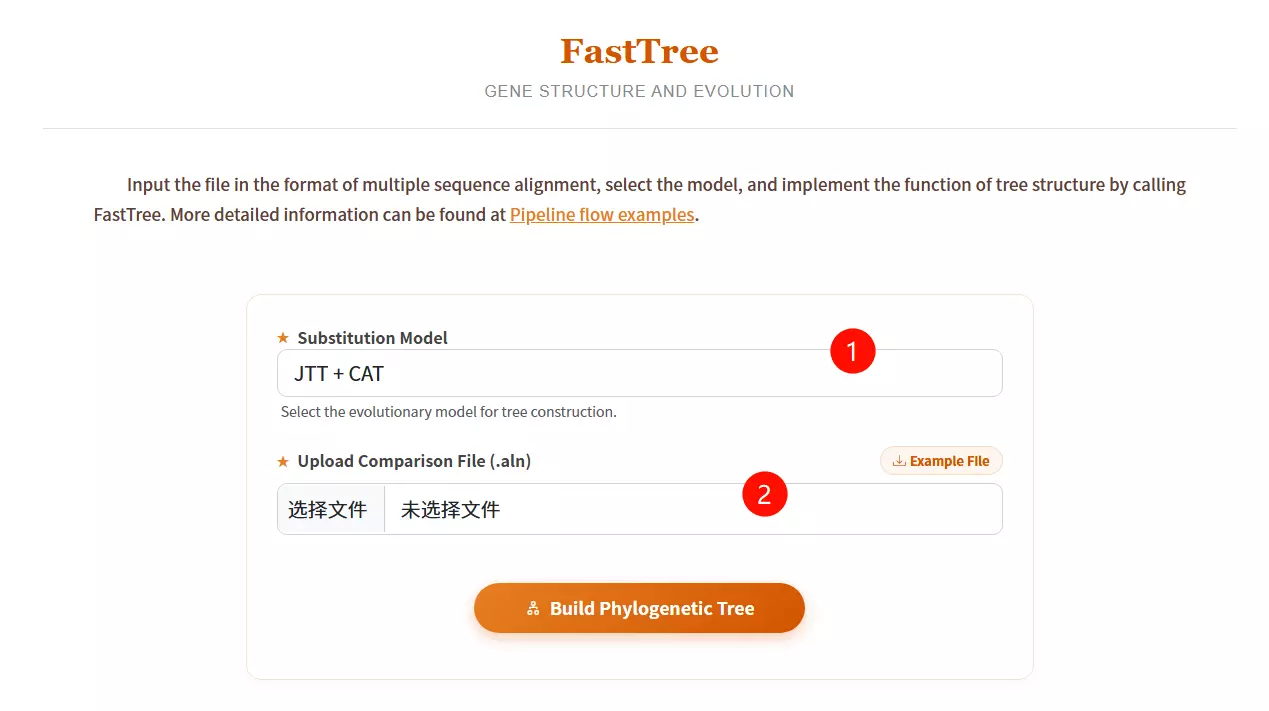
1.Select the Substitution Model Choose the appropriate evolutionary model (e.g., JTT+CAT or GTR+CAT) from the dropdown menu for tree construction.
2.Upload the Comparison File Click to upload the multiple sequence alignment file (usually in FASTA or .aln format) required for the analysis.
3.Click the "Build Phylogenetic Tree" button Submit the form to execute FastTree and generate the phylogenetic tree structure.
# 1. Install Ruby and dependencies
sudo apt-get install ruby gem ruby-dev

# 2. Install SequenceServer gem
sudo gem install sequenceserver

# 3. Prepare Database (Example: Copying to server)
# scp /local/dbindex user@ip:/home/db

# 4. Run SequenceServer (pointing to database directory)
sequenceserver -m -d /db
1. Enter the target sequence to be matched
2. Select the corresponding database
3. Enter the required parameters
4. Click the submit button
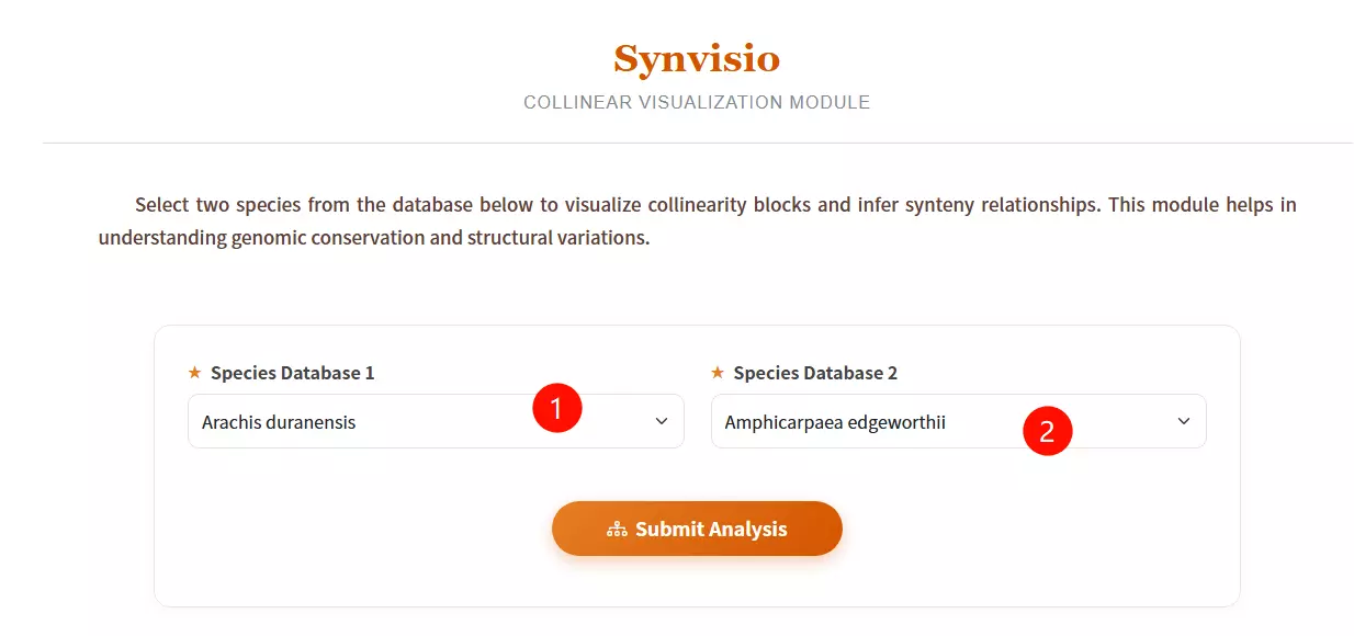
1.Select Species Database 1 Choose the reference species from the first dropdown menu (e.g., Arachis duranensis) to define the base genome for comparison.
2.Select Species Database 2 Choose the target species from the second dropdown menu to analyze collinearity blocks and synteny relationships against the first species.
3.Click the "Submit Analysis" button Submit the form to initiate the Synvisio calculation and generate the visualization results.
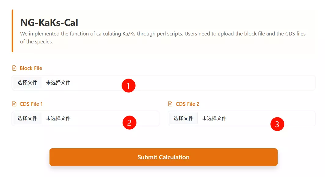
1.Upload the Synteny Block File Click to upload the file containing the collinearity blocks or orthologous gene pairs for the species being analyzed (e.g., .txt or .block format).
2.Upload the First Species CDS File Click to upload the coding sequence file for the first species (must be in FASTA or CDS format).
3.Upload the Second Species CDS File Click to upload the coding sequence file for the second species (must be in FASTA or CDS format).
4.Click the "Run Calculation" button Submit the form to initiate the pipeline and calculate the Ka/Ks ratios for the provided sequences.
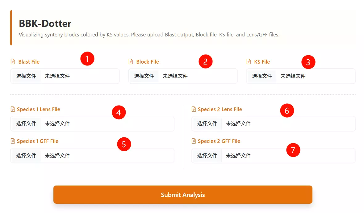
1.Upload the BLAST file Click to upload the sequence alignment result file (usually in tabular format) representing the homology search between the two species.
2.Upload the Block file Click to upload the synteny block file (e.g., generated by MCScanX) that defines the collinear regions between the genomes.
3.Upload the Ks file Click to upload the file containing the calculated Ks (synonymous substitution rate) values for the gene pairs.
4.Upload Species 1 Lens file Click to upload the chromosome length file (Lens file) for the first species (Species 1) to define the genomic coordinates.
5.Upload Species 2 Lens file Click to upload the chromosome length file (Lens file) for the second species (Species 2) to define the genomic coordinates.
6.Upload Species 1 GFF file Click to upload the General Feature Format (GFF) file containing gene annotation information for the first species.
7.Upload Species 2 GFF file Click to upload the General Feature Format (GFF) file containing gene annotation information for the second species.
8.Click the "Run Analysis" button Submit the form to process the data and generate the Ks dotplot visualization.
# a. Change to the path for installing GSDS 2.0 and unpack the tar package.
cd $PATH2INSTALL_GSDS
tar -zxvf gsds_v2.tar.gz

# b. Modify the authentication of task directories and log file
cd $PATH2INSTALL_GSDS/gsds_v2
mkdir task task/upload_file
chmod 777 task/
chmod 777 task/upload_file/
chmod a+w gsds_log

# c. Link CGI commands in directory gcgi_bin to the commands in your system
cd $PATH2INSTALL_GSDS/gsds_v2/gcgi_bin
ln -s -f seqretsplit
ln -s -f est2genome
ln -s -f bedtools
ln -s -f rsvg-convert

# d. Configure Apache2 for accessing GSDS 2.0
# (Follow specific Apache configuration steps for your server environment)
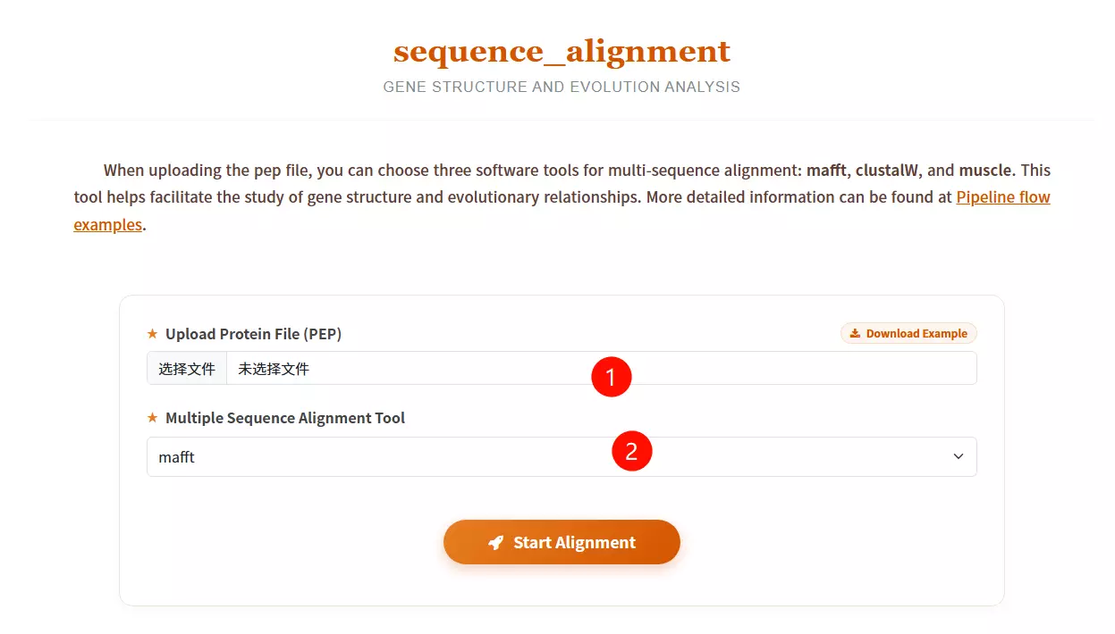
1.Upload the Protein File (PEP) Click to upload the file containing the protein sequences you want to align (must be in FASTA or PEP format).
2.Select the Multiple Sequence Alignment Tool Choose the desired alignment software from the dropdown menu: mafft (known for speed), muscle (high accuracy), or clustalw2 (classic algorithm).
3.Click the "Start Alignment" button Submit the form to initiate the alignment process and analyze the evolutionary relationships between the sequences.
unzip PhyML-3.1.zip
mv PhyML-3.1 /opt/biosoft/
ln -s /opt/biosoft/PhyML-3.1/PhyML-3.1_linux64 /opt/biosoft/PhyML-3.1/PhyML
echo 'PATH=$PATH:/opt/biosoft/PhyML-3.1/' >> ~/.bashrc
source ~/.bashrc
# Standard Command:
PhyML -i proteins.phy -d aa -b 1000 -m LG -f m -v e -a e -o tlr

# Parameter Explanation:
# -i : sequence file name (input)
# -d : data type (nt for nucleotide, aa for amino acid). Default: nt
# -b : bootstrap replicates (int)
# -m : substitution model (e.g., LG, GTR)
# -f : equilibrium frequencies (e, m, or fA,fC,fG,fT)
# -v : proportion of invariant sites (prop_invar)
# -a : gamma shape parameter
# -o : optimize parameters (tlr)
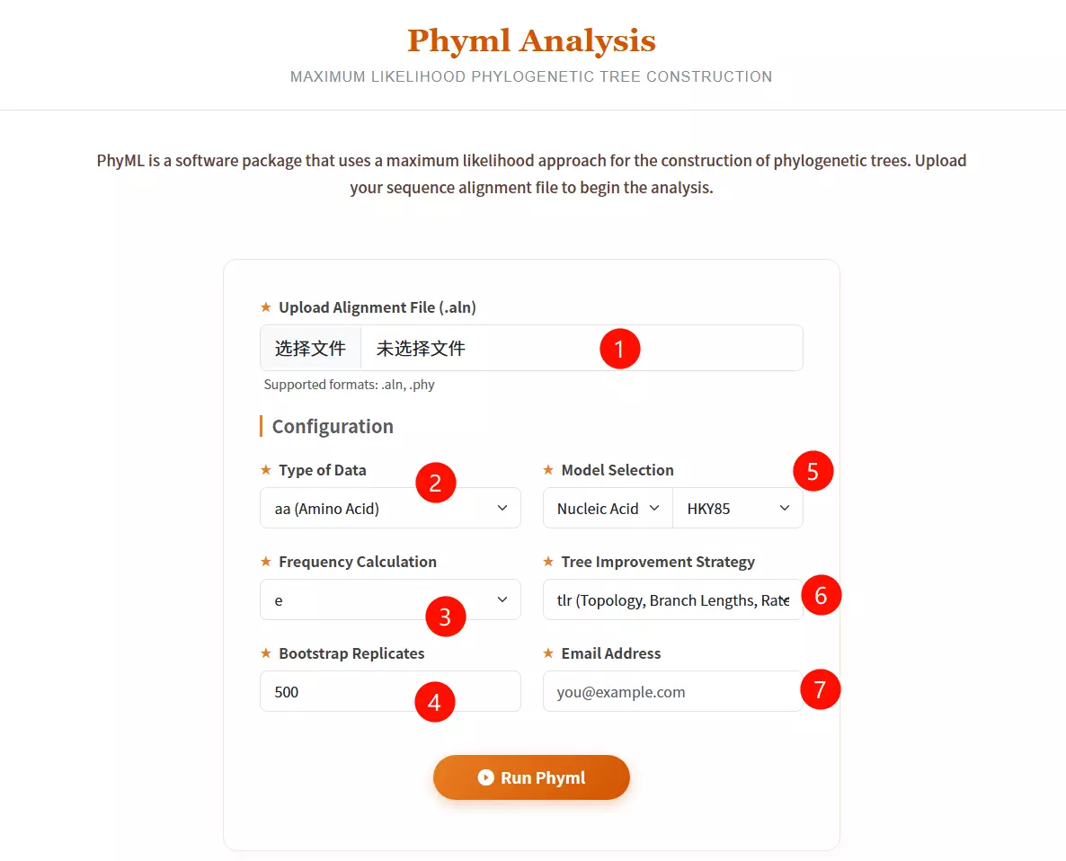
1.Upload Alignment File Click to upload the sequence alignment file (supported formats: .aln, .phy) containing the aligned sequences for analysis.
2.Select Type of Data Choose the data type of your sequences: aa (Amino Acid), nt (Nucleotide), or generic from the dropdown menu.
3.Select Model Category Choose between "Nucleic Acid" or "Protein" in the first model selection box to filter the available evolutionary substitution models.
4.Select Substitution Model Choose the specific evolutionary model (e.g., HKY85, GTR for nucleotides; LG, WAG for proteins) from the second dropdown menu.
5.Select Frequency Calculation Choose the method for calculating equilibrium frequencies (e.g., e, m, fa, fC, fG, fT) to estimate nucleotide or amino acid frequencies.
6.Select Tree Improvement Strategy Choose the parameters to be optimized during tree search: Topology (t), Branch Lengths (l), and/or Rate Parameters (r).
7.Input Bootstrap Replicates Enter the number of bootstrap replicates (default is 500) to assess the reliability of the phylogenetic tree branches.
8.Enter Email Address Input a valid email address to receive the results and notifications once the analysis is complete.
9.Click the "Run Phyml" button Submit the form to start the maximum likelihood analysis and tree construction process.
class sequence_run2(object):
    def __init__(self, place):
        self.id_list = []
        self.place = place

    def new_prot(self):
        new_prot = open(f'{path_get}/file_keep/{self.place}/new_pro.txt', 'w')
        for line in SeqIO.parse(f'{path_get}/file_keep/{self.place}/protein.fasta', 'fasta'):
            if line.id in self.id_list:
                new_prot.write('>' + str(line.id) + '\n' + str(line.seq) + '\n')

    def new_cds(self):
        new_cds = open(f'{path_get}/file_keep/{self.place}/new_cds.txt', 'w')
        for line in SeqIO.parse(f'{path_get}/file_keep/{self.place}/gene.fasta', 'fasta'):
            if line.id in self.id_list:
                new_cds.write('>' + str(line.id) + '\n' + str(line.seq) + '\n')

    def new_gff(self):
        new_gff = open(f'{path_get}/file_keep/{self.place}/new_gff.txt', 'w')
        gff_file = open(f'{path_get}/file_keep/{self.place}/gff.fasta', 'r')
        for line in gff_file:
            gff_id = line.split()[1]
            if gff_id in self.id_list:
                new_gff.write(line)

    def main(self):
        id_file = open(f'{path_get}/file_keep/{self.place}/id.fasta', 'r')
        for line in id_file.readlines():
            self.id_list.append(line.split()[0])
            self.new_prot()
            self.new_cds()
            self.new_gff()
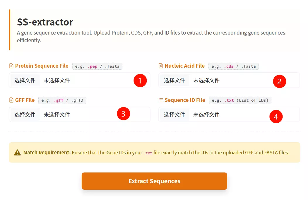
1.Upload the ID List File Click to upload a text file containing the list of specific IDs you want to extract (format: one ID per line).
2.Upload the Protein Sequence File Click to upload the protein sequence file in FASTA format (optional, but at least one data file is required).
3.Upload the Gene/CDS Sequence File Click to upload the coding sequence (CDS) file in FASTA format (optional).
4.Upload the GFF / Table File Click to upload the GFF or table file; the tool will extract lines where the second column matches your IDs (optional).
5.Click the "Filter & Download ZIP" button Submit the form to process the files and download the extracted records as a ZIP archive.
def format_fasta_run(place, file_name, patten, patten_end, file_last):
    SeqIO.convert(
        f"{path_get}/file_keep/{place}/{file_name}.{file_last}",
        f"{patten}",
        f"{path_get}/file_keep/{place}/{file_name}.{patten_end}",
        f"{patten_end}"
    )
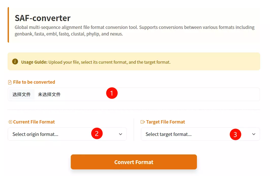
1.Upload the Sequence File Click to upload the biological sequence file containing the data you want to convert.
2.Select the Input Format Choose the specific format that matches your uploaded file (e.g., FASTA, GenBank, EMBL) from the first dropdown menu.
3.Select the Output Format Choose the desired target format you wish to convert your file into (e.g., Phylip, Nexus, Tabular) from the second dropdown menu.
4.Click the "Convert & Download" button Submit the form to initiate the conversion process and download the result.
def quchong_run(place):
    id_list = []
    new_file = open(f'{path_get}/file_keep/{place}/new.fasta', 'w')
    for line in SeqIO.parse(f'{path_get}/file_keep/{place}/1.fasta', 'fasta'):
        if line.id not in id_list:
            id_list.append(line.id)
            new_file.write(">" + str(line.id) + "\n" + str(line.seq) + "\n")
    new_file.close()
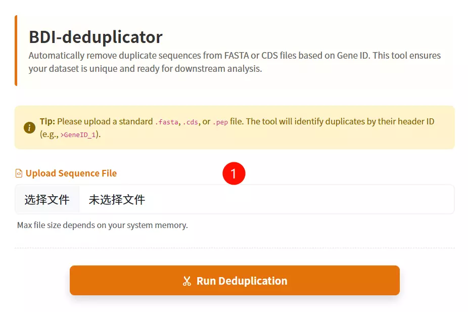
1.Upload the FASTA File Click to upload the sequence file containing the records you wish to deduplicate (supports .fasta, .fa, .faa, .fna, or .txt formats).
2.Click the "Deduplicate & Download" button Submit the form to process the file; the tool will filter out duplicate sequences based on their IDs and download the cleaned file.
def extr_row_run(place, row_num, row_name, row_last):
    cmd = f"""
        cd {path_get}/file_keep/{place}
        cut -f {row_num} {row_name}.{row_last} > {row_name}.new.{row_last}
    """
    subprocess.run(cmd, shell=True, check=True)
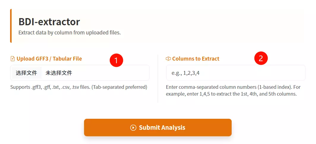
1.Upload the GFF3 / Tabular File Click to upload the structured text file containing the data you want to extract (supports .gff3, .txt, .csv, or .tsv formats).
2.Enter the Columns to Extract Input the specific column numbers you wish to retrieve, separated by commas (e.g., enter "1,4,5" to extract the first, fourth, and fifth columns).
3.Click the "Extract & Download" button Submit the form to process the file and automatically download the new file containing only the selected columns.
def file_merge_run_tools(place):
    cmd = f"""
        cd '{path_get}/file_keep/{place}'
        cat orthomcl/* >> result.txt
    """
    subprocess.run(cmd, shell=True, check=True)
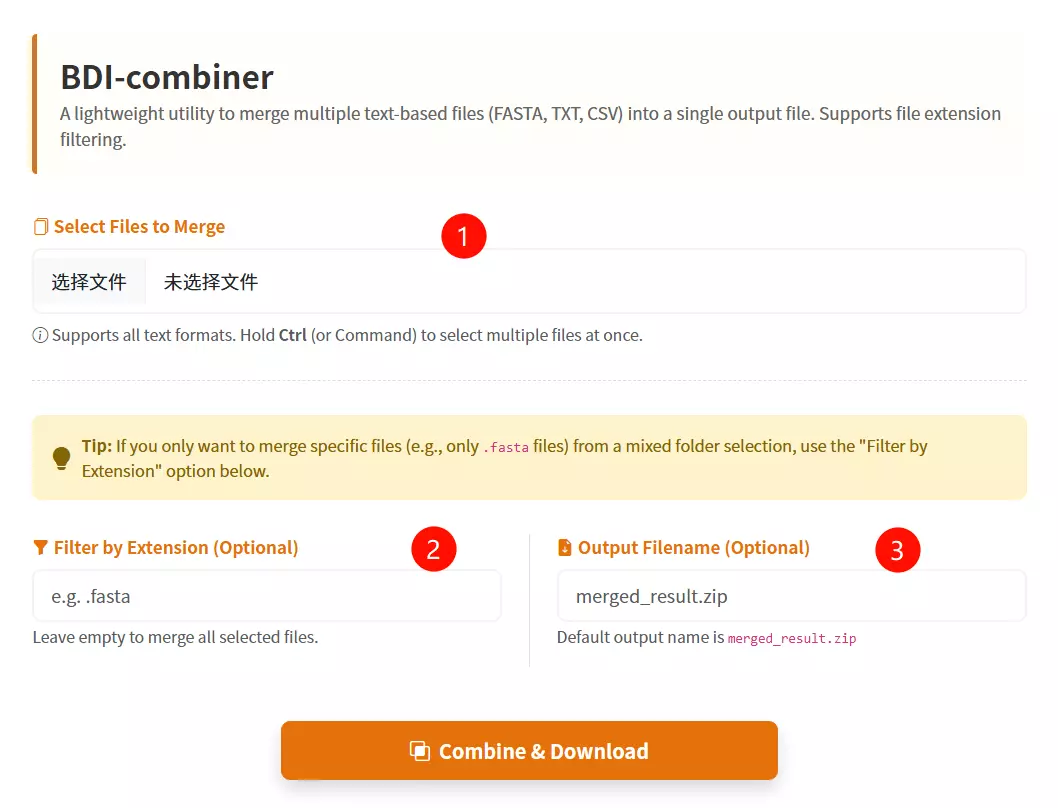
1.Select Multiple Files to Merge Click to browse and select the multiple files you want to combine into a single file (hold Ctrl or Command key to select multiple items).
2.Filter by Extension (Optional) Input a file suffix (e.g., .fasta) if you want to specifically merge only the files with that extension from your selection.
3.Enter Output Filename (Optional) Input the desired name for the resulting merged file (default is merged_result.txt if left empty).
4.Click the "Combine & Download" button Submit the form to merge the selected files and download the consolidated result.
install.packages("shiny")
install.packages("circlize")
install.packages("RColorBrewer")
install.packages("data.table")
install.packages("RLumShiny")

# Bioconductor packages
source("https://bioconductor.org/biocLite.R")
biocLite("GenomicRanges")
# Define the user to spawn R Shiny processes
run_as shiny;

# Define a top-level server which will listen on a port
server {
  # Use port 3838
  listen 3838;

  # Define the location available at the base URL
  location /shinycircos {
    # Directory containing the code and data of shinyCircos
    app_dir /srv/shiny-server/shinyCircos;
    # Directory to store the log files
    log_dir /var/log/shiny-server;
  }
}
# Run the Perl script
perl dotplot.pl
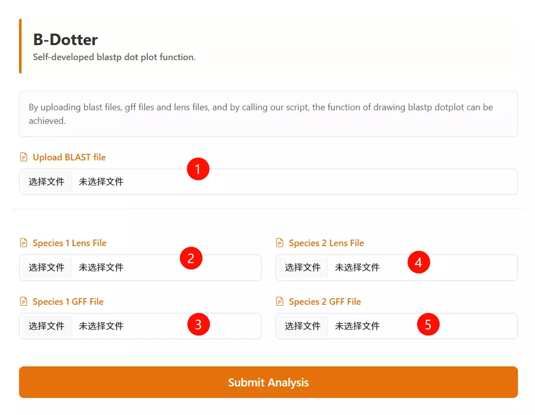
1.Upload the BLAST Output file Click to upload the BLAST result file that contains the alignment information between the two species.
2.Upload the Species 1 Lens file Click to upload the chromosome length file for the first species (usually for the vertical axis).
3.Upload the Species 2 Lens file Click to upload the chromosome length file for the second species (usually for the horizontal axis).
4.Upload the Species 1 GFF file Click to upload the gene feature file (GFF) containing coordinate information for the first species.
5.Upload the Species 2 GFF file Click to upload the gene feature file (GFF) containing coordinate information for the second species.
6.Click the "Run Analysis" button Submit the form to process the uploaded files and generate the synteny dotplot.
# Run the Python script
python dotplot_block.2400.pd.py
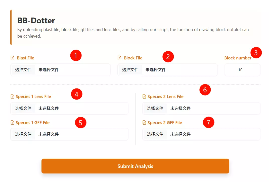
1.Upload the BLAST Output file Click to upload the BLAST result file containing the alignment information between the two species.
2.Upload the Block file Click to upload the synteny block file (usually generated by synteny analysis tools like MCScanX, e.g., .rr.txt).
3.Upload the Species 1 Lens file Click to upload the chromosome length file for the first species (usually displayed on the vertical axis).
4.Upload the Species 2 Lens file Click to upload the chromosome length file for the second species (usually displayed on the horizontal axis).
5.Upload the Species 1 GFF file Click to upload the gene feature file (GFF) containing gene coordinate information for the first species.
6.Upload the Species 2 GFF file Click to upload the gene feature file (GFF) containing gene coordinate information for the second species.
7.Enter the Block Number Input the minimum number of gene pairs required to define a valid synteny block (default is 10).
8.Click the "Run Analysis" button Submit the form to process the data and generate the block dotplot visualization.
# Run the Python script
python corr_dotplot_spc_last.py
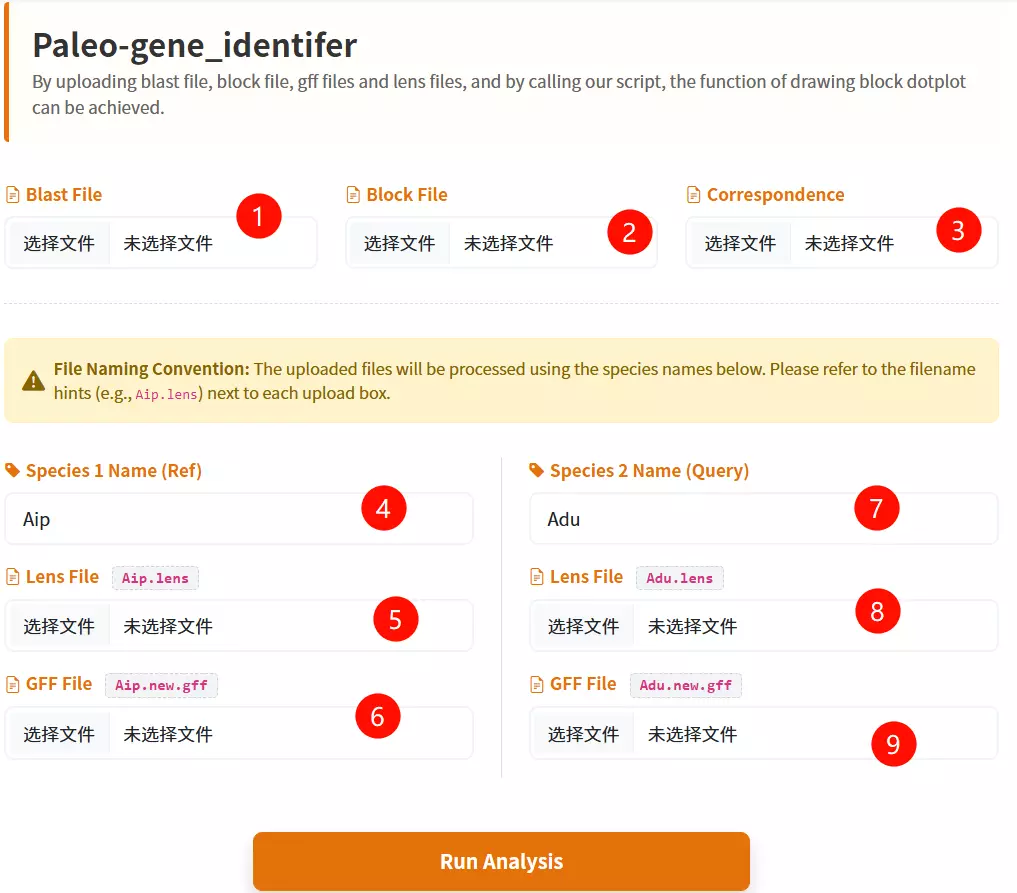
1.Upload the BLAST File Click to upload the BLAST result file containing the alignment information between the two species.
2.Upload the Block File Click to upload the synteny block file (e.g., .block.rr.txt) defining the collinear regions.
3.Upload the Correspondence File Click to upload the correspondence file that maps the relationship between the genomes (e.g., .corr.txt).
4.Enter Species 1 Name Input the short abbreviation for the first species (e.g., Aip) used in the analysis.
5.Upload Species 1 Lens File Click to upload the chromosome length file for the first species.
6.Upload Species 1 GFF File Click to upload the gene feature file (GFF) containing gene coordinates for the first species.
7.Enter Species 2 Name Input the short abbreviation for the second species (e.g., Adu) used in the analysis.
8.Upload Species 2 Lens File Click to upload the chromosome length file for the second species.
9.Upload Species 2 GFF File Click to upload the gene feature file (GFF) containing gene coordinates for the second species.
10.Click the "Run Analysis" button Submit the form to start the synteny inference and evolutionary analysis process.
# Run the Python script
python baoliu.py
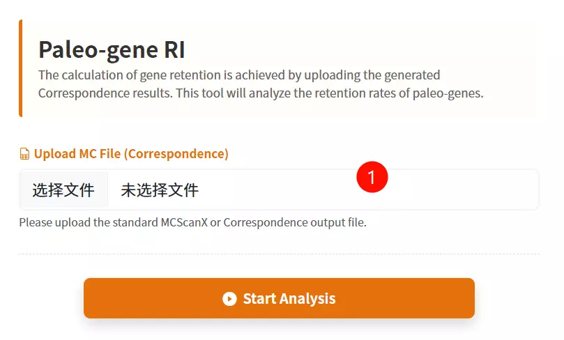
1.Upload the MC File Click to upload the Correspondence (MC) file containing the gene mapping information required for retention analysis.
2.Enter Email Address Input a valid email address to receive the analysis results once the processing is complete.
3.Click the "Submit Analysis" button Submit the form to start the gene retention calculation process.
# Run the Python script
python lost.py
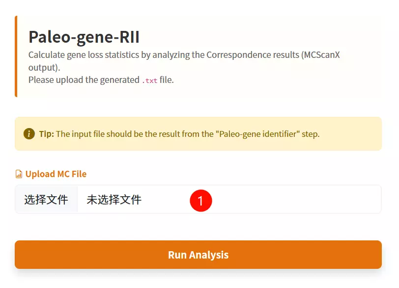
1.Upload the MC File Click to upload the Correspondence result file (usually a .txt file) containing the gene mapping information required to calculate gene loss.
2.Click the "Submit Analysis" button Submit the form to initiate the statistical calculation of paleo-gene loss.
cd DupGen_finder
make
chmod 775 DupGen_finder.pl
chmod 775 DupGen_finder-unique.pl
chmod 775 set_PATH.sh
source set_PATH.sh
# 1. Prepare GFF files (Spd: Experimental, Ath: Control)
cat Spd.bed | sed 's/^/Spd-/g' | awk '{print $1"\t"$4"\t"$2"\t"$3}' > Spd.gff
cat Ath.bed | sed 's/^/Ath-Chr/g' | awk '{print $1"\t"$4"\t"$2"\t"$3}' > Ath.gff
sed -i 's/Chr0/Chr/g' Spd.gff
cat Spd.gff Ath.gff > Spd_Ath.gff

# 2. BLAST Search
# Build DB and Blast for Spd (Self)
makeblastdb -in Spd.pep -dbtype prot -title Spd -parse_seqids -out Spd
blastp -query Spd.pep -db Spd -evalue 1e-10 -max_target_seqs 5 -outfmt 6 -out Spd.blast

# Build DB and Blast for Ath (Reference)
makeblastdb -in Ath.pep -dbtype prot -title Ath -parse_seqids -out Ath
blastp -query Ath.pep -db Ath -evalue 1e-10 -max_target_seqs 5 -outfmt 6 -out Ath.blast

# Combine Results
mkdir Spd_Ath
cat Spd.blast Ath.blast > Spd_Ath.blast

# 3. Run DupGen_finder
# General mode (-t: target, -c: control/outgroup)
DupGen_finder.pl -i $PWD -t Spd -c Ath -o ${PWD}/Spd_Ath/results1

# Strict mode
DupGen_finder-unique.pl -i $PWD -t Spd -c Ath -o ${PWD}/Spd_Ath/results2
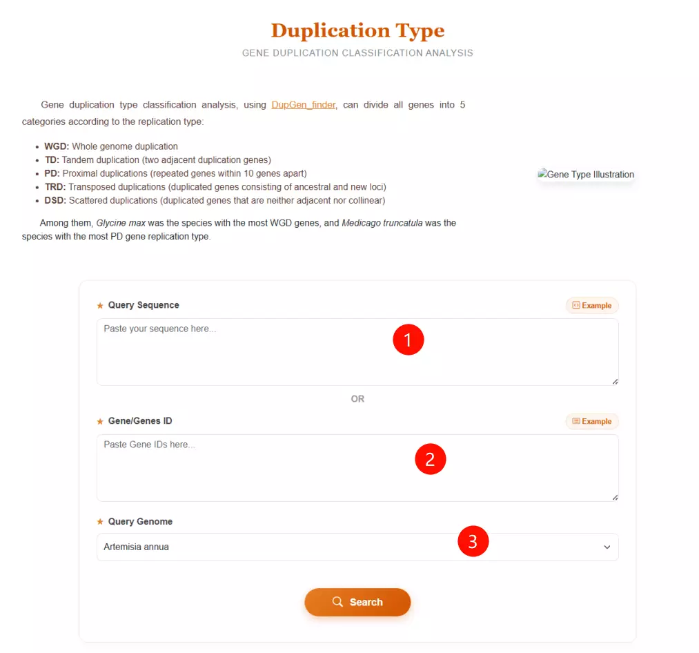
1.Input the Query Sequence Paste your query sequence in FASTA format into the first text area to identify duplication types based on sequence similarity.
2.Input the Gene IDs Alternatively, if you already have the gene identifiers, paste the list of Gene IDs (e.g., Aann1g00011) into the second text area (skip Step 1 if using this option).
3.Select the Query Genome Choose the specific species from the dropdown menu (e.g., Artemisia annua, Vitis vinifera) to serve as the reference for duplication classification.
4.Click the "Search" button Submit the form to process the data and categorize the genes into duplication types (WGD, TD, PD, TRD, DSD).
# Run the Python script with the configuration file
python .\run.py excircle -c excircle.conf
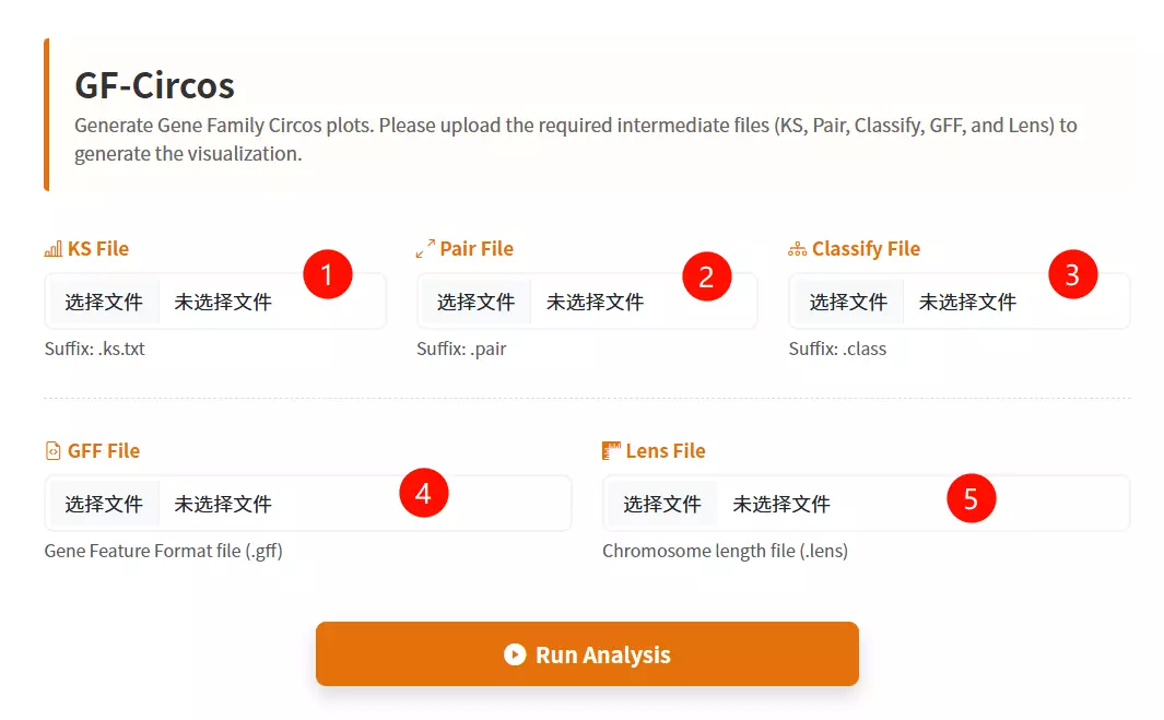
1.Upload the KS File Click to upload the file containing the Ks (synonymous substitution rate) values for the gene pairs.
2.Upload the Pair File Click to upload the file listing the specific gene pairs to be visualized.
3.Upload the Classify File Click to upload the classification file that categorizes the gene pairs (usually by duplication type or family).
4.Upload the GFF File Click to upload the Gene Feature File (GFF) containing the chromosomal coordinate information for the genes.
5.Upload the Lens File Click to upload the chromosome length file required to draw the backbone of the Circos plot.
6.Click the "Draw Circos" button Submit the form to process the uploaded data and generate the circular visualization.
# I. Convert SRA data to fastq format using fasterq-dump
fasterq-dump --split-3 *.sra

# II. Use fastQC to evaluate the quality of fastq files
fastqc *fq

# III. Trimming (Remove adapters, prune bases, filter low quality)
# Double-ended (PE) sequencing:
trimmomatic PE -threads 4 -phred33 *_1.fastq.gz *_2.fastq.gz *_1_clean.fq *_1_unpaired.fq *_2_clean.fq *_2_unpaired.fq \
 ILLUMINACLIP:TruSeq3-PE.fa:2:30:10 LEADING:20 TRAILING:20 SLIDINGWINDOW:4:20 MINLEN:50

# Single-ended (SE) sequencing:
trimmomatic SE -threads 4 -phred33 *.fastq.gz *_clean.fq \
 ILLUMINACLIP:TruSeq3-SE.fa:2:30:10 LEADING:20 TRAILING:20 SLIDINGWINDOW:4:20 MINLEN:50

# IV. Build an index of the reference genome
hisat2-build -p 3 *.fa *.index

# V. Align fastq sequences to the reference genome
# Double-ended (PE):
hisat2 --new-summary --rna-strandness RF -p 10 -x *.index -1 *_1_clean.fq -2 *_2_clean.fq -S *.sam
# Single-ended (SE):
hisat2 --new-summary --rna-strandness R -p 10 -x *.index -U *_clean.fq -S *.sam

# VI. Convert SAM to BAM and Sort
samtools sort -o *.bam *.sam

# VII. Quantitative analysis of gene expression
stringtie -e -A *.out -p 4 -G *.gtf -o *.gtf *.bam
# 1. Process genome files (Index FASTA)
samtools faidx Psa.fasta

# 2. Process GFF3 files (Sort, Zip, and Index)
# Sort and tidy the GFF3 file
gt gff3 -sortlines -tidy -retainids Psa.gff > Psa.sorted.gff

# Compress with bgzip
bgzip Psa.sorted.gff

# Index with tabix
tabix Psa.sorted.gff.gz
# 1. Download and Extract
wget https://ftp.ebi.ac.uk/pub/software/unix/iprscan/5/5.61-93.0/interproscan-5.61-93.0-64-bit.tar.gz
tar -pxvzf interproscan-5.61-93.0-*-bit.tar.gz
cd interproscan-5.61-93.0

# 2. Set Environment Variables
export PATH=`pwd`:$PATH

# * Note: Software relies on Java 11 or above
export PATH=/home/public/tools/jdk-17.0.1/bin:$PATH
# A. For Protein Sequences
interproscan.sh -cpu 40 -d anno.dir -dp -i protein.fa

# B. For Nucleic Acid (Transcript) Sequences
interproscan.sh -cpu 40 -d anno.dir -dp -t n -i transcripts.fa

# Parameter Explanation:
# -cpu : Number of threads
# -d   : Output directory
# -dp  : Disable pre-calculated match lookup (force local calculation)
# -i   : Input sequence file
# -t   : Sequence type (n for nucleic acid, p for protein [default])
1.Upload the Sequence File Click to upload the raw data file you wish to process (supports formats such as FASTA, TXT, or CSV).
2.Input the Find String (Old Name) Enter the specific character string or pattern currently exists in the file that you want to target (e.g., "scaffold_").
3.Input the Replacement String (New Name) Enter the new character string that will replace the target text defined in the previous step (e.g., "Chr").
4.Click the "Run Calculation & Download" button Submit the form to execute the find-and-replace operation and initiate the download of the processed file.
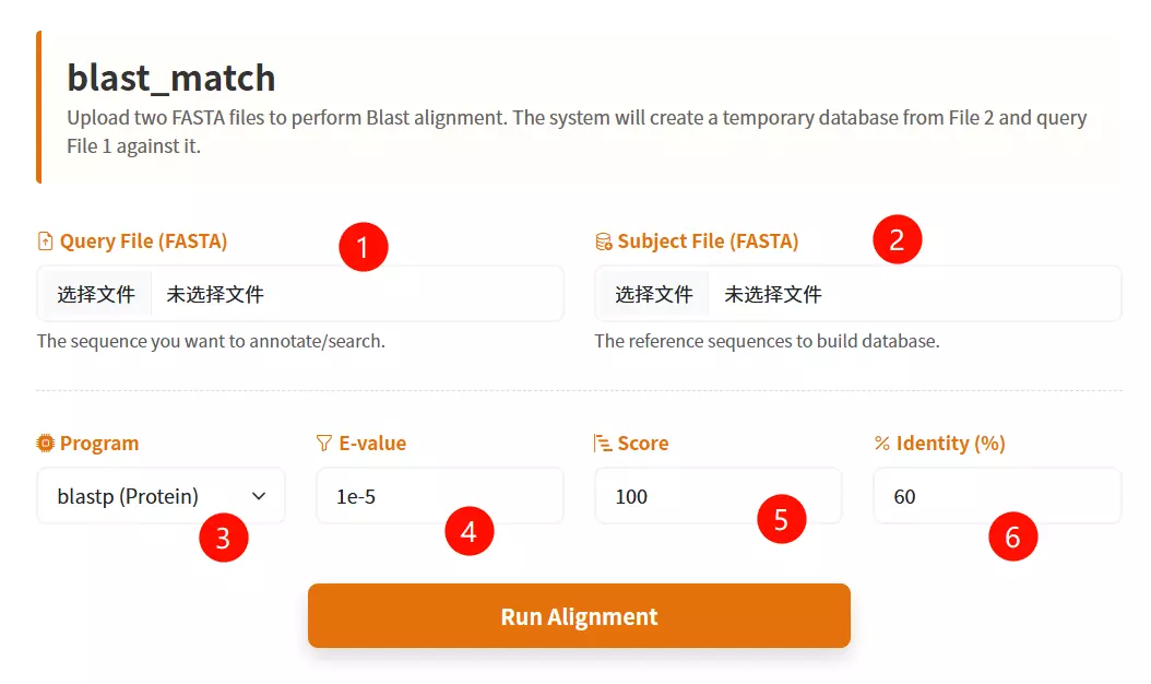
1.Upload the Target Database file Click the upload area to select and upload your sequence file in FASTA format (e.g., .fasta).
2.Select the Blast Subroutine Choose the appropriate alignment algorithm from the dropdown menu: use "blastp" for protein sequences or "blastn" for nucleotide sequences.
3.Select the Species Database Choose the specific target organism from the provided species list to perform the alignment against.
4.Enter the E-value threshold Input the expectation value cutoff (default is 1e-5) to filter out statistically insignificant alignment results.
5.Input the Score Value Enter the minimum alignment score required for a match to be retained (default is 100).
6.Input the Identity Value Enter the minimum percentage of sequence identity required (default is 60) to define a valid match.
7.Click the "Run Blast Match" button Submit the form to initiate the homology search and alignment process.
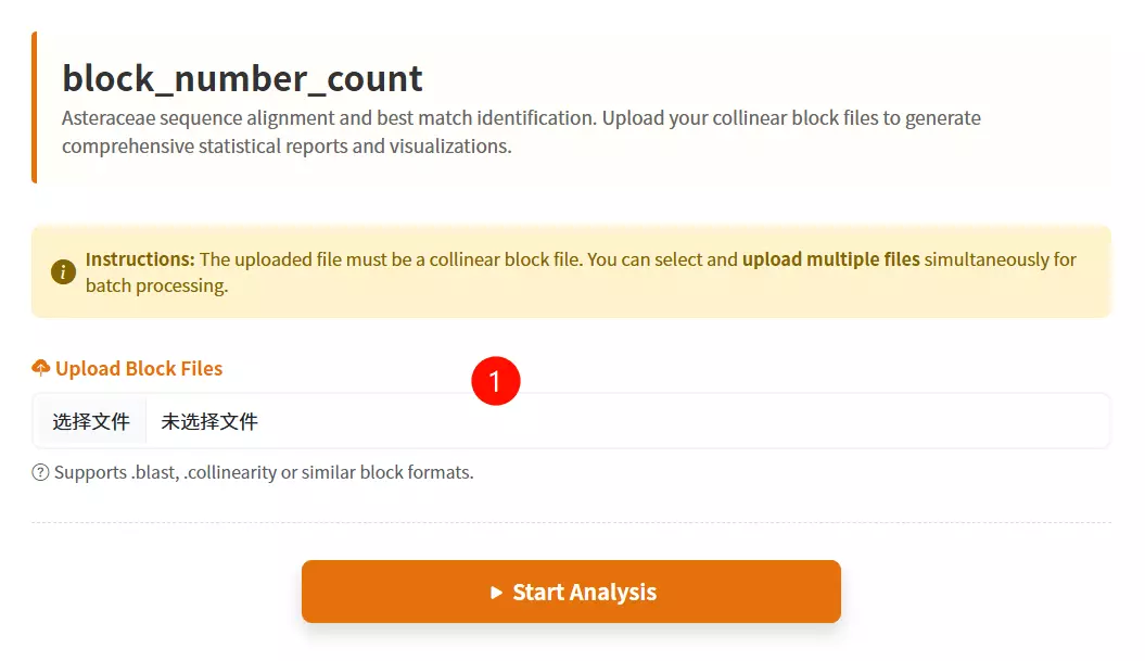
1.Upload the Collinear Block files Click to select and upload the data files you want to analyze (supports .blast and .txt formats); you can select multiple files at once.
2.Click the "Submit Analysis" button Submit the form to execute the block number statistical calculation and initiate the result download.
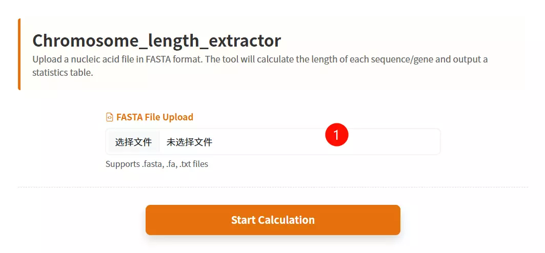
1.Upload the Sequence File Click to upload the nucleic acid sequence file (e.g., CDS or Chromosome sequences) you want to analyze (must be in FASTA format).
2.Click the "Submit Analysis" button Submit the form to calculate the length of each sequence and generate the statistics table.
3.Download the Result Table (Optional) Once the calculation is complete and the table is displayed, click this button to save the ID and Length data as a text file.
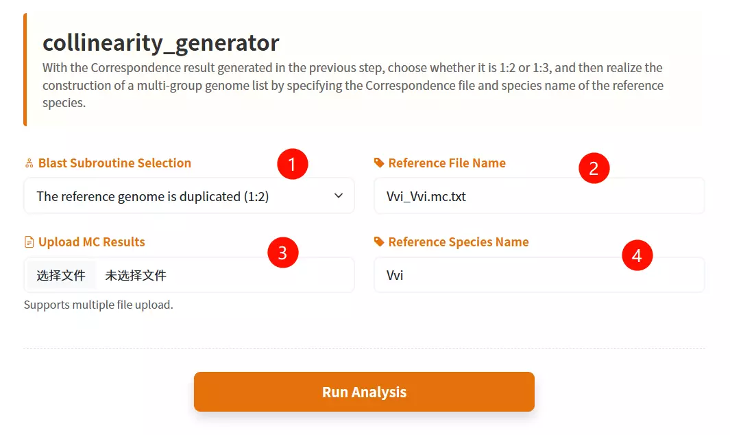
1.Select the Reference Genome Ploidy Choose the appropriate ploidy ratio (Duplicated 1:2 or Triplicated 1:3) from the dropdown menu to define the structure of the reference genome.
2.Upload the MC Results files Click to upload the correspondence result files generated from previous analysis steps (supports multiple files or compressed archives).
3.Enter the Reference File Name Input the specific filename of the reference species' self-alignment result (e.g., "Vvi_Vvi.mc.txt").
4.Enter the Reference Species Name Input the abbreviation or identifier for the reference species (e.g., "Vvi").
5.Click the "Generate List" button Submit the form to construct the multi-group genome list and initiate the evolutionary analysis process.
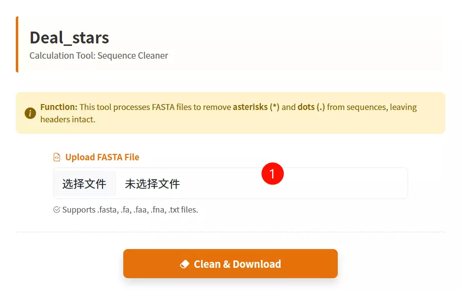
1.Upload the Sequence File Click to upload the FASTA format file (supports .fasta, .fa, .txt, etc.) containing the sequences from which you want to remove asterisks (*) and dots (.).
2.Click the "Clean & Download" button Submit the form to process the file, stripping out the unwanted characters while preserving headers, and initiate the download of the cleaned file.
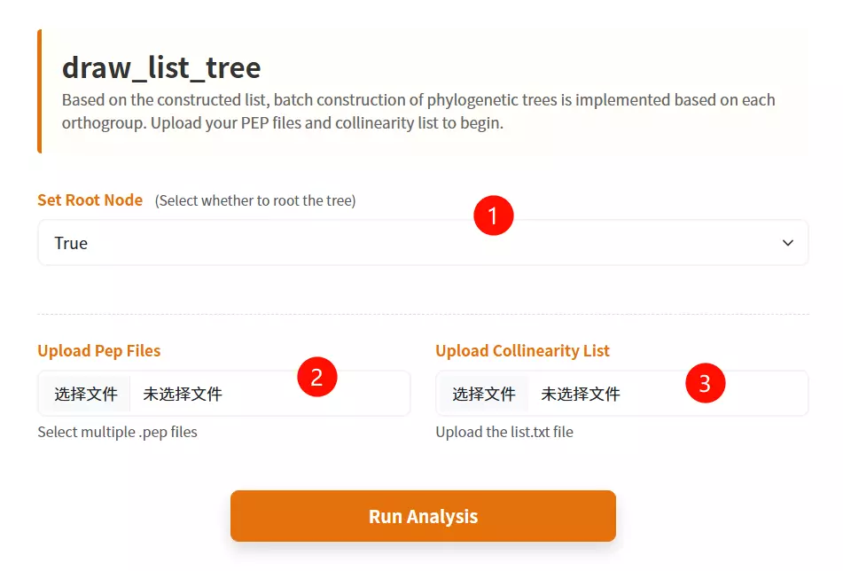
1.Set the Root Node option Select "True" or "False" from the dropdown menu to determine whether the generated phylogenetic trees should be rooted.
2.Upload the Protein Sequence (PEP) files Click to upload the protein sequence files for the relevant species (multiple files can be selected simultaneously).
3.Upload the Collinearity List file Click to upload the specific text file containing the orthogroup or collinearity list constructed in the previous analysis.
4.Click the "Construct Trees" button Submit the form to automate the batch construction of phylogenetic trees based on the uploaded inputs.
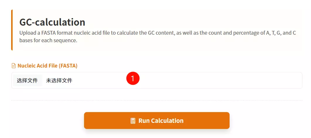
1.Upload the FASTA File Click to upload the nucleic acid sequence file (e.g., CDS sequences) you want to analyze (must be in FASTA format).
2.Click the "Start Calculation" button Submit the form to calculate the base composition (A, T, C, G) and generate the statistics table.
3.Download the Result Table (Optional) Once the calculation is complete and the table is displayed, click this button to save the detailed statistical data as a text file.
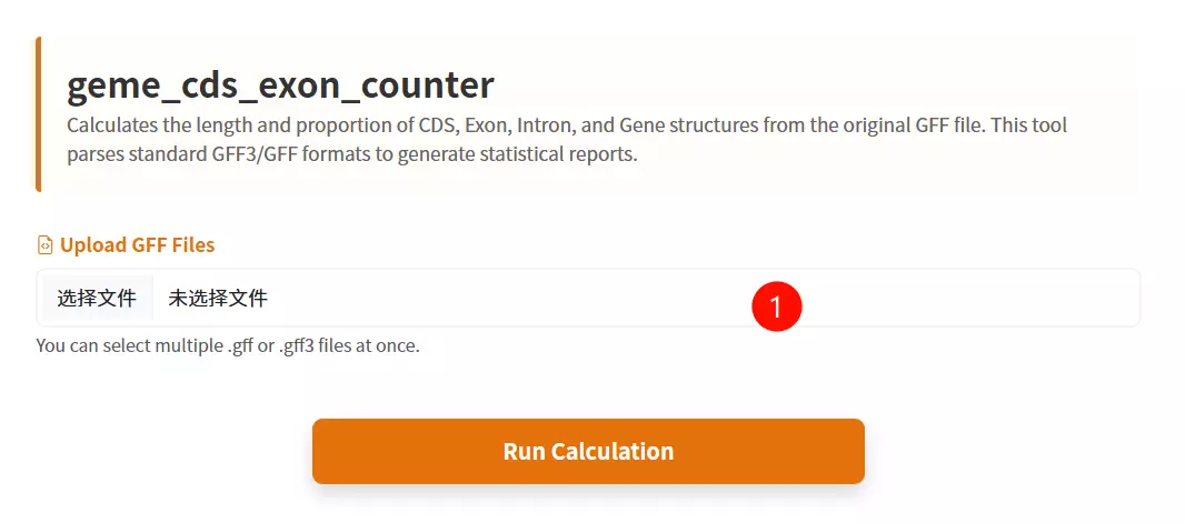
1.Upload the GFF annotation files Click to upload the gene feature files you want to analyze (supports GFF format, and multiple files can be uploaded simultaneously).
2.Click the "Submit & Calculate" button Submit the form to calculate the statistics for genes, exons, introns, and CDS, and to generate the results table.
3.Download the Result Table (Optional) Once the calculation is complete and the table is displayed, click this button to save the detailed statistical metrics as a text file.

1.Upload the GFF File Click to upload the gene annotation file containing structural information (must be in GFF format).
2.Upload the Highlight File Click to upload the file containing the list of specific gene IDs you wish to highlight in the diagram.
3.Input the Chromosome Position Enter the specific chromosome number or identifier where the target genes are located (e.g., "1").
4.Input the Starting Position Enter the numeric start coordinate on the chromosome to define the beginning of the drawing range (e.g., "1200").
5.Input the Termination Position Enter the numeric end coordinate on the chromosome to define the end of the drawing range (e.g., "162713").
6.Click the "Draw Structure" button Submit the form to generate and visualize the gene structure diagram based on the input parameters.
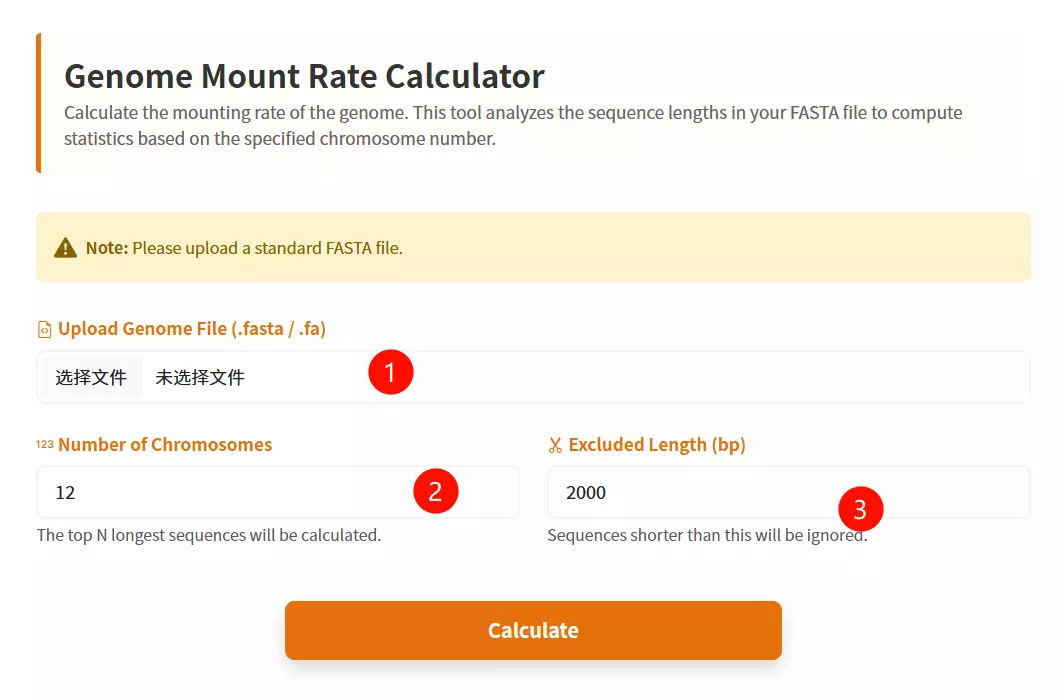
1.Upload the Genomic File Click to upload the genome sequence file you wish to analyze (must be in FASTA format and less than 200MB).
2.Input the Number of Chromosomes Enter the total count of chromosomes expected in the genome (default is 12).
3.Input the Exclusion Length Threshold Enter the minimum sequence length value; sequences shorter than this threshold (e.g., small scaffolds or contigs) will be excluded from the calculation (default is 2000).
4.Click the "Calculate" button Submit the form to perform the genome mount rate calculation and generate the results table.
5.Download the Result Table (Optional) Once the calculation is complete and the table is displayed, click this button to save the genome mount rate statistics as a text file.
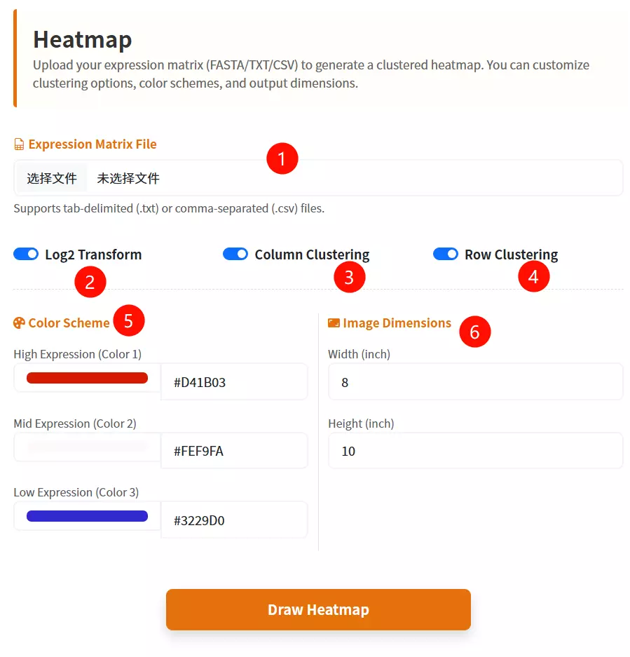
1.Upload the Target Database file Click to upload the gene expression data file (labeled as FASTA format in the interface).
2.Configure Log2 Transformation Check the box to apply a Log2 transformation to your data values (default is checked).
3.Set Column Clustering Check the box to enable hierarchical clustering for the data columns (default is checked).
4.Set Row Clustering Check the box to enable hierarchical clustering for the data rows (default is checked).
5.Select the First Color Choose a color from the picker or enter a hex code for the first part of the gradient (default is #D41B03).
6.Select the Second Color Choose a color from the picker or enter a hex code for the middle part of the gradient (default is #FEF9FA).
7.Select the Third Color Choose a color from the picker or enter a hex code for the last part of the gradient (default is #3229D0).
8.Enter Image Width Input the desired numerical width for the generated heatmap image (default is 8).
9.Enter Image Height Input the desired numerical height for the generated heatmap image (default is 10).
10.Click the "Draw Heatmap" button Submit the form to generate and visualize the gene expression heatmap.
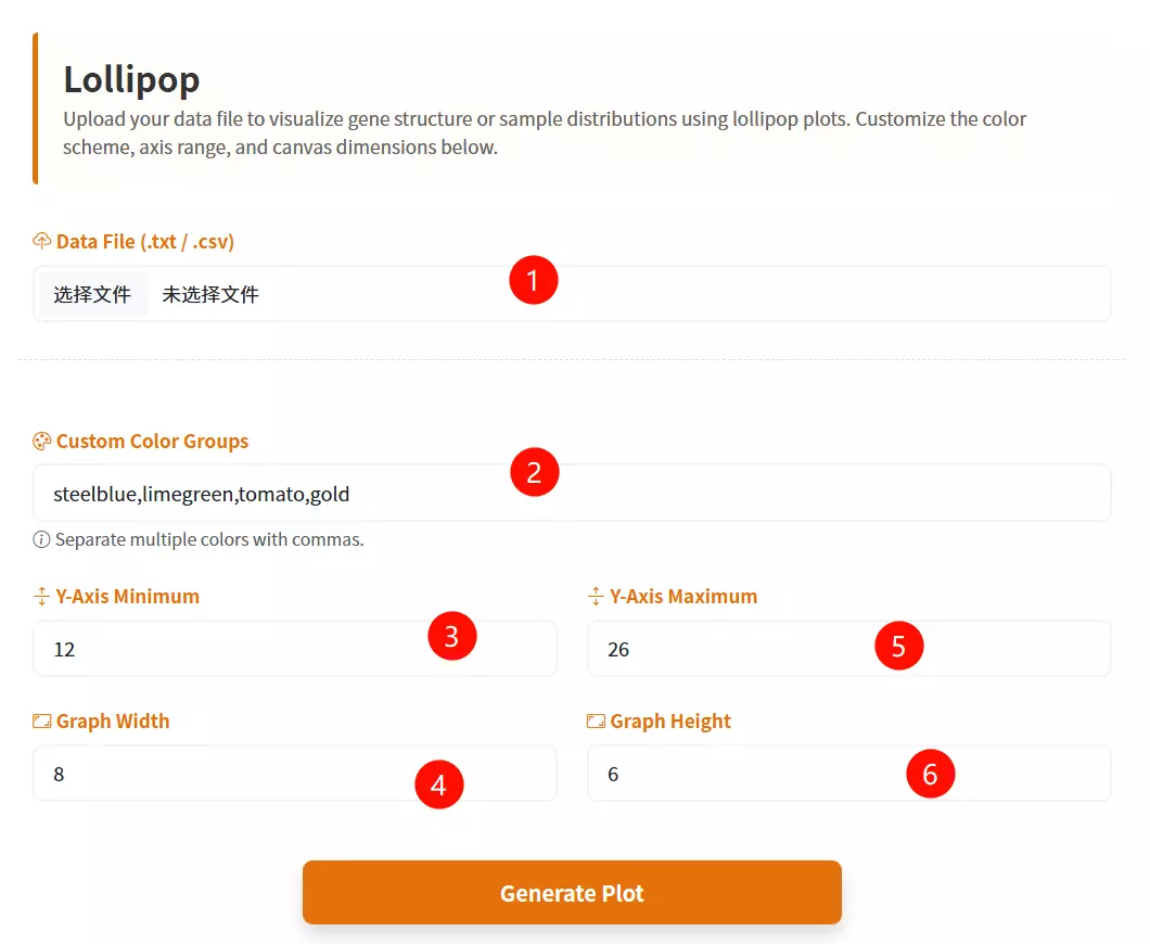
1.Upload the Data File Click to upload the text-based data file containing your dataset (expected format includes columns for Species, Value, and Group).
2.Select the Sort Order Choose the desired sorting method for the data values from the dropdown menu (e.g., Descending or Ascending).
3.Select the Base Color Click the color picker interface to define the primary color used for the data points (dots).
4.Adjust the Dot Size Drag the slider to set the specific pixel diameter for the data points (ranging from 5 to 30 pixels).
5.Click the "Plot Lollipop" button Submit the configured form to generate and render the interactive Lollipop Chart.
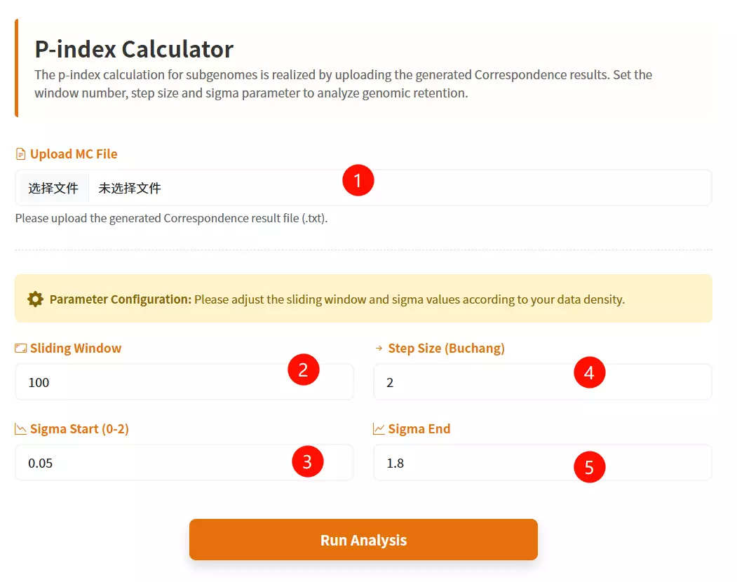
1.Upload the MC File Click to upload the correspondence result file containing collinearity data (e.g., a text file generated from previous correspondence analysis).
2.Enter the Sliding Window Input the window size for the analysis (default is 100) to define the range of genes considered in each step.
3.Enter the Step Size Input the numerical increment for the moving window (default is 2) to control the granularity of the analysis.
4.Input the Sigma Start Value Enter the starting threshold for the sigma parameter (between 0 and 2, default is 0.05).
5.Input the Sigma End Value Enter the ending threshold for the sigma parameter (between 0 and 2, default is 1.8).
6.Click the "Run Analysis" button Submit the form to start the P-Index calculation and generate the evolutionary trend analysis.

1.Select the Target Species Choose the specific species code (e.g., Arachis duranensis - Adu) from the dropdown menu to define the source genome for sequence retrieval.
2.Input the Gene ID List Enter the specific gene identifiers (one per line, e.g., Adu01g03207) into the text area, or click the "Example" button to load sample data.
3.Click the "Submit Analysis" button Submit the form to fetch the CDS and protein sequences corresponding to the entered IDs.
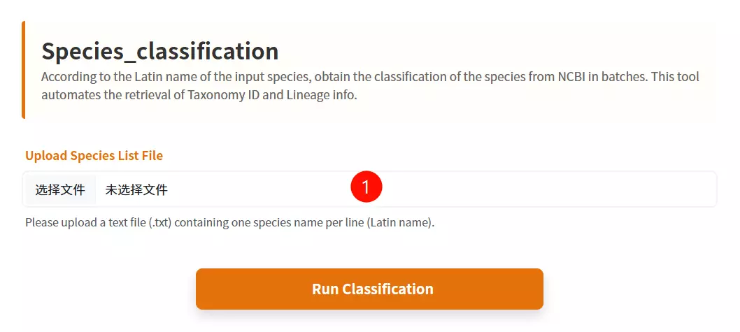
1.Upload the Species List file Click to upload the text file containing the Latin names of the species you want to classify (one species name per line).
2.Click the "Get Classification" button Submit the form to retrieve the taxonomic classification information from NCBI in batches.
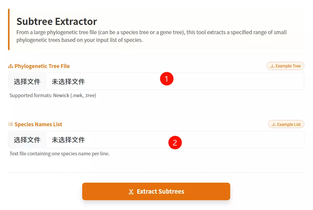
1.Upload the Phylogenetic Tree file Click to upload the master tree file (usually in Newick format) containing the complete evolutionary relationships.
2.Upload the Species List file Click to upload the text file containing the specific list of species or gene names you want to extract from the main tree.
3.Click the "Extract Subtrees" button Submit the form to isolate and generate the smaller phylogenetic tree based on your provided list.
# Create a virtual environment named “jcvi” using conda
conda create -y -c bioconda -c conda-forge -n jcvi python=3.10

# Activate the Environment
conda activate jcvi

# Install the last tool
conda install -c bioconda last

# Install JCVI
pip install jcvi

# Verify Installation
jcvi --version
python -m jcvi.compara.catalog ortholog species1 species2
python -m jcvi.graphics.dotplot species1.species2.anchors
python -m jcvi.compara.synteny screen --minspan=30 --simple species1.species2.anchors species1.species2.anchors.new
python -m jcvi.graphics.karyotype seqids layout
# Error 1: Command ‘lastdb/lastal’ not found
# Solve 1: conda install -c bioconda last

# Error 2: LaTeX/dvipng missing (plotting error)
# Solve 2: sudo apt-get install texlive texlive-latex-extra texlive-fonts-recommended dvipng
# Go to Alexis github repository and download the latest RAxML version. When the download is completed type:
unzip standard-RAxML-master.zip

# This will create a directory called standard-RAxML-master
# Change into this directory by typing
cd standard-RAxML-master

# Initially, we will need to compile the RAxML executables.
# To obtain the sequential version of RAxML type:
make -f Makefile.gcc

# this will generate an executable called raxmlHPC. If you then want to compile an additional version of RAxML make always sure to type rm *.o before you use another Makefile. Assume, we are using a laptop with two cores:
1. make -f Makefile.gcc
2. rm *.o
3. make -f Makefile.SSE3.gcc
4. rm *.o
5. make -f Makefile.PTHREADS.gcc
6. rm *.o
7. make -f Makefile.SSE3.PTHREADS.gcc

# Once we are done with compiling the code we can execute it locally:
./raxmlHPC

# or copy all the executables into our local directory of binary files:
cp raxmlHPC* ~/bin/

# To get an overview of available commands type:
raxmlHPC -h
raxmlHPC-PTHREADS-AVX2 -f a -x 123456 -p 123456 -s example.fasta -m GTRGAMMA -N 1000 -n output
raxmlHPC-PTHREADS-AVX2 -f a -x 123456 -p 123456 -s example.fasta -m PROTGAMMAAUTO -N 1000 -n output
# Error 1: RAxML_bestTree.alignment: No such file or directory
# Solve 1: Check the RAxML_info.alignment log file to troubleshoot the cause of the error.

# Error 2: Out of Memory
# Solve 2: Reduce the number of threads (e.g., from 16 to 8 threads), use the GTRCAT model (more memory-efficient than GTRGAMMA), and run in stages (first perform ML search, then Bootstrap).
# Create and activate a virtual environment
conda create -n of3_env python=3.12
conda activate of3_env

# Install OrthoFinder (including core dependencies: diamond, mcl, fastme)
conda install orthofinder

# Verify Installation (Check Version Number)
orthofinder --version
orthofinder -f ./proteins/ -S diamond -M msa -T raxml -t 8

# -f ./proteins/: Specify input directory (containing FASTA files for proteins across all species);
# -S diamond: Use diamond for fast sequence alignment (default, 10-100 times faster than blastp);
# -M msa: Infer gene trees using multiple sequence alignment (MSA) methods;
# -T raxml: Construct gene trees using RAxML (requires prior installation of RAxML; raxmlHPC-AVX2 version recommended);
# -t 8: Accelerate alignment using 8 threads (adjust based on CPU core count).
# Error 1: ImportError: No module named numpy or numpy.core.multiarray failed to import
# Solve 1: conda install numpy
export PYTHONPATH="$CONDA_PREFIX/lib/python3.10/site-packages:$PYTHONPATH"

# Error 2: external program called by OrthoFinder returned an error code: 255
# Solve 2:
# Step 1: Check if RAxML is installed: `which raxmlHPC-AVX2`
# Step 2: Modify OrthoFinder's `config.json` changing the RAxML command to:
# "raxml": {
#   "program_type": "tree",
#   "cmd_line": "raxmlHPC-AVX2 -m PROTGAMMALG -p 12345 -s INPUT -n IDENTIFIER -w PATH > /dev/null",
#   "output_filename": "PATH/RAxML_bestTree.IDENTIFIER"
# }
# Step 3: Manually test the RAxML command.

# Error 3: Input file format not recognized or Sequence length mismatch
# Solve 3: Check file format: `head ./proteins/Human.faa`. Unify sequence length using MAFFT or Muscle.
# Download KofamScan software and database
wget ftp://ftp.genome.jp/pub/tools/kofam_scan/kofam_scan-1.3.0.tar.gz
tar -xzvf kofam_scan-1.3.0.tar.gz

# Download the KEGG Database
wget ftp://ftp.genome.jp/pub/db/kofam/profiles.tar.gz
wget ftp://ftp.genome.jp/pub/db/kofam/ko_list.gz
gunzip ko_list.gz
tar -xzvf profiles.tar.gz

# Configure Environment Variables (Add KofamScan to PATH)
echo 'export PATH=/path/to/kofam_scan-1.3.0/bin:$PATH' >> ~/.bashrc
source ~/.bashrc
exec_annotation -o output.txt -f mapper -p /path/profiles -k /path/ko_list -E 1e-5 --cpu 6 --tmp-dir tmp_dir input.faa
# Error 1: No such file or directory: 'hmmsearch' or LoadError: cannot load such file -- parallel
# Solve 1: conda install hmmmer parallel

# Error 2: Profile database not found
# Solve 2: exec_annotation --profile /custom/path/profiles

# Error 3: Invalid input format
# Solve 3: Check file format: `head input.faa` (ensure it starts with `>` and the sequence is in protein alphabet)
# Create and activate the virtual environment (Python 3.8+ recommended)
conda create -n trimal_env -y
conda activate trimal_env

# Install trimAl (Bioconda channel)
conda install -c bioconda trimAl
trimal -in input.pep -out output.out -gt 0.3
# Error 1: g++: command not found(Linux/macOS)
# Solve 1: sudo apt-get install build-essential  # Ubuntu
# sudo yum groupinstall "Development Tools"      # CentOS

# Error 2: No such file or directory.
# Solve 2: Add the trimAl executable to the PATH.
# Download
wget https://circos.ca/distribution/circos-0.69-10.tgz
tar xzf circos-0.69-10.tgz
cd circos-0.69

# Test
cd circos-0.69/example/
../bin/circos -conf etc/circos.conf

# Check
circos -modules
circos -conf circos.conf -outputdir ./output -outputfile circos.png
# Error 1: Can't locate <Module>.pm in @INC.
# Solve 1: conda install -c bioconda perl-gd.

# Error 2: Configuration file error.
# Solve 2: Add karyotype = <path/to/karyotype.txt> to circos.conf.

# Error 3: Invalid data format
# Solve 3:
# Step 1: Verify that the data file is tab-delimited;
# Step 2: Ensure each line contains four columns (chromosome ID, start position, end position, value)
# Create and activate the virtual environment
conda create -n pal2nal -y -c bioconda perl bioperl
conda activate pal2nal

# Install Pal2NAL
conda install -c bioconda pal2nal
pal2nal.pl pep.aln nuc.fa -output fasta -nogap -codontable universal > nuc.aln

pal2nal.pl -i sample.id pep.aln nuc.fa -output axt -codontable universal

pal2nal.pl -i sample.id pep.aln nuc.fa -codeml
# Error 1: Can't locate Bio/SeqIO.pm in @INC.
# Solve 1: conda install -c bioconda perl-bioperl.

# Error 2: ERROR: inconsistency between the following pep and nuc seqs.
# Solve 2: Check file IDs and standardize ID formats using seqkit or a Python script.

# Error 3: The output result is empty.
# Solve 3:
# Step 1: Verify FASTA format: head nuc.fa (must begin with >, sequence consists of DNA letters).
# Step 2: Ensure each protein corresponds to a unique DNA sequence ID.
# Download
wget http://research-pub.gene.com/gmap/src/gmap-gsnap-2023-12-01.tar.gz
tar -zxvf gmap-gsnap-2023-12-01.tar.gz
cd gmap-gsnap-2023-12-01

# Configuration and Compilation
./configure --prefix=/path/to/install
make -j4
make install
gmap_build -D /path/gmapdb -d species genome.fa
gmap -D /path/gmapdb -t 10 -d species -f gff3_gene input.cds >output.gff
gmap -t 10 -d species -f gff3_gene input.fa > output.gff
# Error 1: Can't locate Bio/SeqIO.pm in @INC.
# Solve 1: conda install -c bioconda perl-bioperl.

# Error 2: chromosome lengths not found.
# Solve 2: samtools faidx reference.fa.

# Error 3: No paths found for <Seq ID>
# Solve 3: Downgrade to a stable version (e.g., 2017-11-15). Verify that the sequence format is FASTA.
# Download source code
git clone https://github.com/gpertea/gffread
cd gffread

# Compile and install
make release # Generate executable files in the current directory
sudo cp gffread /usr/local/bin/ # Add to system path
gffread input.gff3 -T -o output.gtf
gffread input.gtf -o output.gff3
gffread input.gff3 -g genome.fa -x cds.fa
gffread input.gff3 -g genome.fa -y protein.fa
# Error 1: Can't locate Bio/SeqIO.pm in @INC.
# Solve 1: conda install -c bioconda perl-bioperl.

# Error 2: Invalid GFF/GTF format
# Solve 2: Verify that the file conforms to the GFF3/GTF specification using `gffread -h`.

# Error 3: Sequence ID not found in genome file.
# Solve 3: Ensure that the IDs in the genome FASTA files match the seqids in the annotation file.